
Research article · 2022 · Full text
International Journal of Statistics and Applied MathematicsReliability for Weibull Distribution using Ms-Excel
Volume 7(5) · Pages 27–30 · DOI: 10.22271/maths.2022.v7.i5a.878 ↗
Research areasProbabilistic and Robust Engineering Design
Abstract
Author-writtenThe weibull distribution is mostly used in reliability analysis life data analysis due to its versatility. Depending on the values of the parameters, the weibull distribution can be used to model a variety of life behaviors. The three parameter weibull distribution can estimate the probability of null wind speed and gives greater weight to low wind speeds. We also discuss least square method of estimation problems and hypothesis testing issues, with the emphasis on graphical methods and some weibull analysis software are also provided. The analysis is also applicable in the design stage and in-service time as well and it is not only limited to the production stage. Now, the techniques to perform the Weibull analysis process are done by statistical software programs.
Summary
Source-checkedPlain-language reading of the full paper, prepared with AI and checked against the text. Each point links to the authors' own words.
Why it matters
- The Weibull distribution is widely utilized in life data and reliability analysis because it is versatile. View evidence ↗
- The distribution's ability to model various life behaviors depends on the specific values of its parameters. View evidence ↗
- Weibull analysis is useful across multiple phases, including the design stage and in-service time, rather than just during production. View evidence ↗
The question
- The study aims to demonstrate how to determine reliability, median ranks, and the unreliability function using a specific dataset. View evidence ↗
What they did
- The authors outline a specific multi-step procedure in MS-Excel to calculate median ranks and linearize the unreliability function. View evidence ↗
- Linear regression is used to estimate Weibull parameters, where the slope of the line represents the shape parameter. View evidence ↗
What they found
- For the provided dataset, the estimated shape parameter (β) is 3.104 and the characteristic life (ɳ) is 30.399. View evidence ↗
What it means
- The authors conclude that their objective was achieved by successfully defining median ranks, Weibull parameter estimates, and reliability representations in MS-Excel based on time to failure. View evidence ↗
- The research concludes by outlining the status of the studied extruder using the derived reliability analysis. View evidence ↗
Visual summary
2 visualsIllustrations explain the paper; charts are replotted from the paper's own table values.
Linear Regression for Weibull Parameters
AI-generated conceptual illustration (A scatter plot of data points on a coordinate plane). It explains the idea and does not show study data.
View source evidence ↗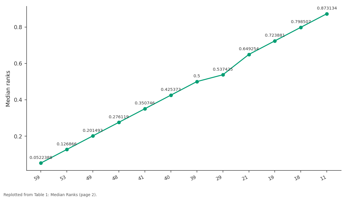
Median ranks: 59 vs 53 vs 49 vs 48 vs 41
Replotted from Table 1 (page 2) of the original paper. Every bar is the paper's own table value.
View source evidence ↗Figures & tables
From the original paper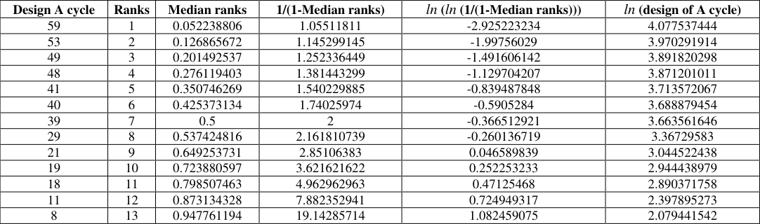 Table 1
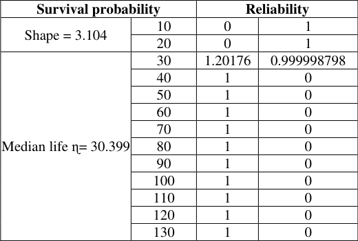 Table 2
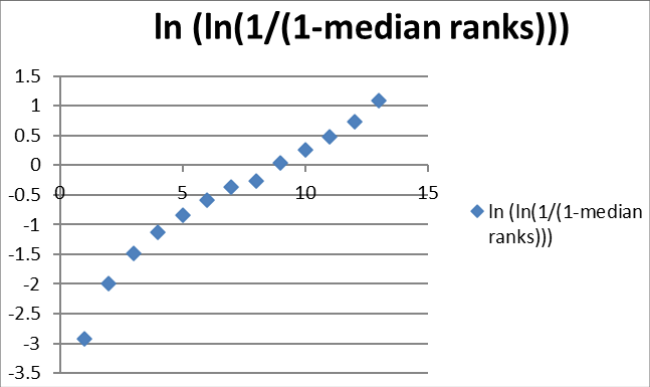 Figure 1
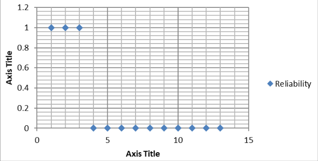 Figure 2
Introduction
The used in reliability engineering, medical research, quality control, finance and climatology. Time –to-failure, such as the probability that a part fails after one, two (or) more years. Described by Three parameters Shape (β) Scale (ɳ) Threshold parameters (or) location (y) The three- parameter weibull distribution expression The probability density function is F(T) = 𝑇−𝛾)𝛽 ɳ (𝑇−𝛾|ɳ)𝛽−1𝑒−(ɳ F (T)≥0, T≥0, γ, β >0, ɳ > 0, -∞ < 𝛾< ∞ Weibull reliability metrics The probability distribution function can be used to derive reliability metrics such as the reliability function, failure rate, mean and median. Weibull Reliability function R (T) = 𝑒−(ɳ 𝑇−𝛾)𝛽 R (T) = 𝑒−(ɳ 𝑡)𝛽 When threshold is zero Maths 2022; 7(5): 27-30 G Vijayalakshmi Research scholar, Department of Statistics, Sri Krinadevaraya University, Anantapur, Andhra Pradesh, India K. Pushpanjali Prof., Department of Statistics, Sri Krinadevaraya University, Anantapur, Andhra Pradesh, India G Vijayalakshmi Research scholar, Department of Statistics, Sri Krinadevaraya University, Anantapur, Andhra Pradesh, India https://www.mathsjournal.com 𝑓(𝑇) 𝛽 R (T) decreases for0 < 𝛽< 1 For β = 1, R(T) decreases monotonically but less sharply than for 0 < 𝛽< 1 For β > 1 R (T) decreases as increases Weibull Failurate Function X(T) = ɳ ) 𝛽−1 𝑅(𝑇)= ɳ (𝑇−𝛾 𝑗−0.3 Y =β x – β ln (ɳ) Where M =β (Slope (or) Sharpe parameter) And intercept is equal to b =- β ln (ɳ) Determining the appropriate y plotting positions or the unreliability values We must first determine a value indicating the corresponding unreliability for that failure. The most widely used method is the method of obtaining the median rank for each failure. The median rank is the value that the true probability of failure, Q (t). Should have at the jth failure out of a sample of n units at the 50% confidence level.
Median ranks are calculated using the following equation also known as Benard’s approximation. F (t) = 1 Population with β < 1exhibit a failure rate that decreases with time. Population with β=1 have a constant failure rate. Population with β > 1 has a failure rate that increases with time. Weibull mean life (or) mean time to failure MTTF ₸ = γ + ɳ, ℾ ( 𝛽+ 1) 𝑛+0.4 j is the failure order n is the sample size Illustration solve by using Ms-Excel We have to find out the dependability or reliability, median ranks and unreliability function to the following data. The desired reliability at 400 cycles is 0.90 I e90% of the value to survive at least 400 cycles. 1 ℾ is a function γ is a parameter Where ℾ is the gamma function ℾ(n) = ∫𝑒−𝑥xn-1d x Median life (or) β 50Life Ť = γ + ɳ (ln 2) 𝛽 In these case of the 2- parameter weibull, the c d f (also the unreliability Q (t)) is given by F (t) = Q (t) =1 −𝑒−(ɳ 𝑡)𝛽 This can be linearised by Q (t) =1 −𝑒−(ɳ 𝑡) β 𝑡)𝛽 ln Q (t) =𝑙𝑛 (1 − (𝑒− (ɳ 𝑗−0.3 𝑡)𝛽 ln (1- Q (t))= 𝑙𝑛𝑒−(ɳ Design A cycle 19 41 39 18 8 29 11 59 40 48 53 49 21 Procedure First consider the design A type the data in Excel sheet then rank them 1 to 13 as given table. Using the linearizing the unreliability function. Now, estimate of the proportion of the population that will fail by the number of cycles listed.
This can be done by determining the median rank F (t) = 𝑡 ln (1 – Q(t))=−( ɳ)𝛽 𝑡 ln (-ln (1- Q(t)))=𝛽 (log ( ɳ)) 𝑛+0.4j is the failure cycle & n = 13. Steps to calculated Median ranks values in MS-Excel Step1: Enter the formula = ((B2-0.3/(10+0.4)) Step 2: Then determine 1 / (1-Median ranks) Step 3: Followed by ln (ln (1/(1- Median ranks))) Step 4: Determine in (design of A cycles) ln (ln (1/ (1- Q(t)))=β ln t – β ln (ɳ) This forms Y = M x + b Y = ln (ln (1/ (1- Q(t))) & x = ln t Table 1: Median Ranks Design A cycle Ranks Median ranks 1/(1-Median ranks) ln (ln (1/(1-Median ranks))) ln (design of A cycle) 59 1 0.052238806 1.05511811 -2.925223234 4.077537444 53 2 0.126865672 1.145299145 -1.99756029 3.970291914 49 3 0.201492537 1.252336449 -1.491606142 3.891820298 48 4 0.276119403 1.381443299 -1.129704207 3.871201011 41 5 0.350746269 1.540229885 -0.839487848 3.713572067 40 6 0.425373134 1.74025974 -0.5905284 3.688879454 39 7 0.5 2 -0.366512921 3.663561646 29 8 0.537424816 2.161810739 -0.260136719 3.36729583 21 9 0.649253731 2.85106383 0.046589839 3.044522438 19 10 0.723880597 3.621621622 0.252253233 2.944438979 18 11 0.798507463 4.962962963 0.47125468 2.890371758 11 12 0.873134328 7.882352941 0.724949317 2.397895273 8 13 0.947761194 19.14285714 1.082459075 2.079441542 https://www.mathsjournal.com Fig 1: Median Ranks Fig 2: Reliability When we perform the linear regression the estimate for the weibull parameter comes directly from the slope of the line. Considering the straight line Y = M x + C M = β (Slope (or) shape parameter) ɳ = Characteristics life = (Parameter is (- ratio of intercept to slope)) (- C / β) ∴ 𝛽= 3.104; b = - β ln (ɳ) = ɳ = 30.399 Table 2: Reliability functions and typical graphical representations of reliability analysis. Thus it is possible to state that the objective was successfully achieved.
| Survival probability | — | Reliability | — |
|---|---|---|---|
| Shape = 3.104 | 10 | 0 | 1 |
| 20 | 0 | 1 | |
| Median life ɳ= 30.399 | 30 | 1.20176 | 0.999998798 |
| 40 | 1 | 0 | |
| 50 | 1 | 0 | |
| 60 | 1 | 0 | |
| 70 | 1 | 0 | |
| 80 | 1 | 0 | |
| 90 | 1 | 0 | |
| 100 | 1 | 0 | |
| 110 | 1 | 0 | |
| 120 | 1 | 0 | |
| 130 | 1 | 0 |
Table text extracted from the original PDF; superscript letters are shown inline. The original table image is below.
View original table image
| Design A cycle | Ranks | Median ranks | 1/(1-Median ranks) | ln (ln (1/(1-Median ranks))) | ln (design of A cycle) |
|---|---|---|---|---|---|
| 59 | 1 | 0.052238806 | 1.05511811 | -2.925223234 | 4.077537444 |
| 53 | 2 | 0.126865672 | 1.145299145 | -1.99756029 | 3.970291914 |
| 49 | 3 | 0.201492537 | 1.252336449 | -1.491606142 | 3.891820298 |
| 48 | 4 | 0.276119403 | 1.381443299 | -1.129704207 | 3.871201011 |
| 41 | 5 | 0.350746269 | 1.540229885 | -0.839487848 | 3.713572067 |
| 40 | 6 | 0.425373134 | 1.74025974 | -0.5905284 | 3.688879454 |
| 39 | 7 | 0.5 | 2 | -0.366512921 | 3.663561646 |
| 29 | 8 | 0.537424816 | 2.161810739 | -0.260136719 | 3.36729583 |
| 21 | 9 | 0.649253731 | 2.85106383 | 0.046589839 | 3.044522438 |
| 19 | 10 | 0.723880597 | 3.621621622 | 0.252253233 | 2.944438979 |
| 18 | 11 | 0.798507463 | 4.962962963 | 0.47125468 | 2.890371758 |
| 11 | 12 | 0.873134328 | 7.882352941 | 0.724949317 | 2.397895273 |
| 8 | 13 | 0.947761194 | 19.14285714 | 1.082459075 | 2.079441542 |
Table text extracted from the original PDF; superscript letters are shown inline. The original table image is below.
View original table image
Since all the median ranks, linear regression the estimate for the weibull parameters and reliability representations in MS- Excel sheet of interest were defined based on time to failure. It has been observed that the above calculations, Reliability starts with 1 end with 0. Total failure density is one.
Conclusions
Reliability analysis is determined by based on the above Table (1), Table (2) Fig (1) and Fig (2). This research has outlined the status of the extruder studied in terms of https://www.mathsjournal.com 7. Dekking FM, et al. A Modern Introduction to Probability and Statistics: Understanding Why and How, Springer; c2007. 8.
Hastings NAJ, Peacock B, Evans M. Statistical DistributionEdition 3rd ed., John Wiley &Sons Inc; c2000. 9. Meeker WQ, Escobar LA. Statistical Methods for Reliability Data 1st ed., Wiley-Interscience; c1998. 10.
Meeker WQ, Escobar LA. Statistical Methods for Reliability Data 1st ed., Wiley-Interscience; c1998. 11. Modarres M, Kaminskiy M, Krivtsov V. Reliability engineering and risk analysis, CRC Press; c1999. 12.
Meeker WQ, Escobar LA. Statistical Methods for Reliability Data 1st ed., Wiley-Interscience; c1998. 13. Singpurwalla ND. Reliability and Risk: A Bayesian Perspective 1st ed., Wiley;c2006. 14.
Pabla AS. Electric Power Distribution, 5th Ed., New Delhi, India: Tata Mc G raw Hill Publishing Company Limited; c2008. 15. KolowrockiK. Limit reliability functions of some series- parallel and parallel series systems, Journal of Applied Mathematics and Computation.1994;62:129-151. 16.
Roy B, Allan RN. Reliability Evaluation of power systems, 2nd Ed. Springer, Newdelhi, 2008, 220-221.
References
6 in the original paper- Jiang R, Murthy DNP. A study of Weibull shape Survival probability Reliability Shape = 3.104 10 0 1 20 0 1 parameter: Properties and significance. Reliability Engineering & System Safety. 2011;96(12):1619-26. Doi:10.1016/j.ress.2011.09.003.
- Bauckhage Christian. Computing the Kullback-Leibler Median life ɳ= 30.399 Divergence between two Weibull Distributions, 2013. arXiv:1310.3713 [cs.IT].
- Wind Speed Distribution Weibull- REUK.co.uk. www.reuk.co.uk.
- Liu Chao, White Ryen W,Dumais Susan. Understanding web browsing behaviors through Weibull analysis of dwell time. ACM, 2010-07-19, 379–386. Doi:10.1145/1835449.1835513. ISBN 9781450301534.
- Sharif NawazM, Islam NazrulM. The Weibull distribution as a general model for forecasting technological change". Technological Forecasting and Social Change. 1980;18(3):247-56. Doi:10.1016/0040- 1625(80)90026-8.
- Artin E. The Gamma Function, New York: Holt, Rinehart & Winston; c1964. 30 1.20176 0.999998798 40 1 0 50 1 0 60 1 0 70 1 0 80 1 0 90 1 0 100 1 0 110 1 0 120 1 0 130 1 0
Cited by 3
From OpenAlex, OpenCitations and reference lists read by Scinovex
- Predictive Model for the Nematode (Hysterothylacium aduncum) in Horse Mackerel, Trachurus trachurus From the Black Sea ↗
Hijran Yavuzcan Yıldız, Ercüment Genç, Doğukan Kaya, Bilgenur HARMANŞA YILMAZ · Marine and Life Sciences · 2024
Hysterothylacium aduncum is a parasitic nematode that infects mainly marine fish. The information on the heterogeneity in the aggregation of macroparasites in fish species is still limited, particularly for the Raphidascarid nematode H. aduncum that infects exploitable marine fish species including horse mackerel (Trachurus trachurus). This study aimed to investigate the heterogeneity of the distribution of H. aduncum to understand…
❝ 2PDF - Experimental and dual statistical validation of additively manufactured thermoset CFRP composites: Using a Weibull–SPC framework for reliability assessment ↗
Rajkumar Wagmare, Rahul Harshe, Jaising Pednekar, Phani Kumar Mallisetty, T. Umasankar Patro · Journal of Composite Materials · 2026
Additive manufacturing (AM) of thermoset continuous carbon fiber-reinforced polymer (CFRP) composites offers significant potential for aerospace and defense applications; however, their statistical reliability characteristics remain insufficiently explored. In this study, ten unidirectional laminates were fabricated using an in-house-developed automatic fiber placement-based additive manufacturing (AFP-AM) system under controlled processing parameters. Rheological analysis was conducted to optimize tow-infusion temperature, while scanning electron…
❝ 0 - Weibull Analysis of Flexural Strength and Surface Asymmetry in Soda-Lime Float Glass Under Varying Loading Rates ↗
Oualid Dairi, Habia Mohamed Ilyes, Mohamed Hamidouche, Zahra Malou Hamidouche, Tarek Bali, Akram Zegadi et al. · Journal of Materials Engineering and Performance · 2026
❝ 0