
Research article · 2022 · Full text
International Journal of Statistics and Applied MathematicsEstimation of stress-strength reliability for poisson-exponential distribution under progressive type II censoring
Volume 7(5) · Pages 36–40 · DOI: 10.22271/maths.2022.v7.i5a.880 ↗
Research areasEngineering Diagnostics and Reliability
Abstract
Author-writtenIn this study, we are aiming to estimate the stress-strength reliability, R=P(Y<X) based on progressive type-II censored samples when X and Y are independent random variables from a two parameter Poisson-Exponential distribution with the same scale but different shape parameters. The maximum likelihood and Bayesian approaches are used for estimation of R when the scale parameter is unknown. Next, in order to compare the performance of the proposed estimators, we carry out a Monte Carlo simulation study and one real data set is conducted to observe the performance of the proposed estimators.
Summary
Source-checkedPlain-language reading of the full paper, prepared with AI and checked against the text. Each point links to the authors' own words.
Why it matters
- In reliability and life testing, it is often impractical to observe all failure times due to constraints such as cost, time, and experimental simplicity. View evidence ↗
- Type-II progressive censoring is a widely used method to handle these data collection constraints. View evidence ↗
- Stress-strength reliability focuses on the probability that the strength of a component (X) exceeds the stress applied to it (Y). View evidence ↗
The question
- The study aims to estimate the stress-strength reliability parameter R = P(Y < X) for independent Poisson-Exponential random variables under progressive type-II censoring. View evidence ↗
What they did
- The authors employ both Maximum Likelihood Estimation (MLE) and Bayesian approaches to estimate R when the scale parameter is unknown. View evidence ↗
- Because the likelihood equations lack a closed-form solution, the Newton-Raphson algorithm is used to find the MLEs. View evidence ↗
- Bayesian estimators for R are computed using importance sampling under Squared Error (SEL) and LINEX loss functions. View evidence ↗
- The performance of the estimators was evaluated using a Monte Carlo simulation with 1000 replications. View evidence ↗
What they found
- Simulation results indicate that Bayes estimators have smaller Mean Square Errors (MSEs) compared to Maximum Likelihood Estimators. View evidence ↗
- Among the tested censoring schemes, the (r1, r3) combination yielded the smallest MSE. View evidence ↗
- In a real data set analysis of airplane window strength, the estimated values for R were 0.1986 (MLE), 0.07075 (SEL), and 0.0414 (LINEX). View evidence ↗
What it means
- The authors conclude that Bayes estimators using the LINEX loss function exhibit lower risk than those using the SEL function. View evidence ↗
Visual summary
3 visualsIllustrations explain the paper; charts are replotted from the paper's own table values.
Stress-Strength Concept
AI-generated conceptual illustration (a mechanical steel bolt). It explains the idea and does not show study data.
View source evidence ↗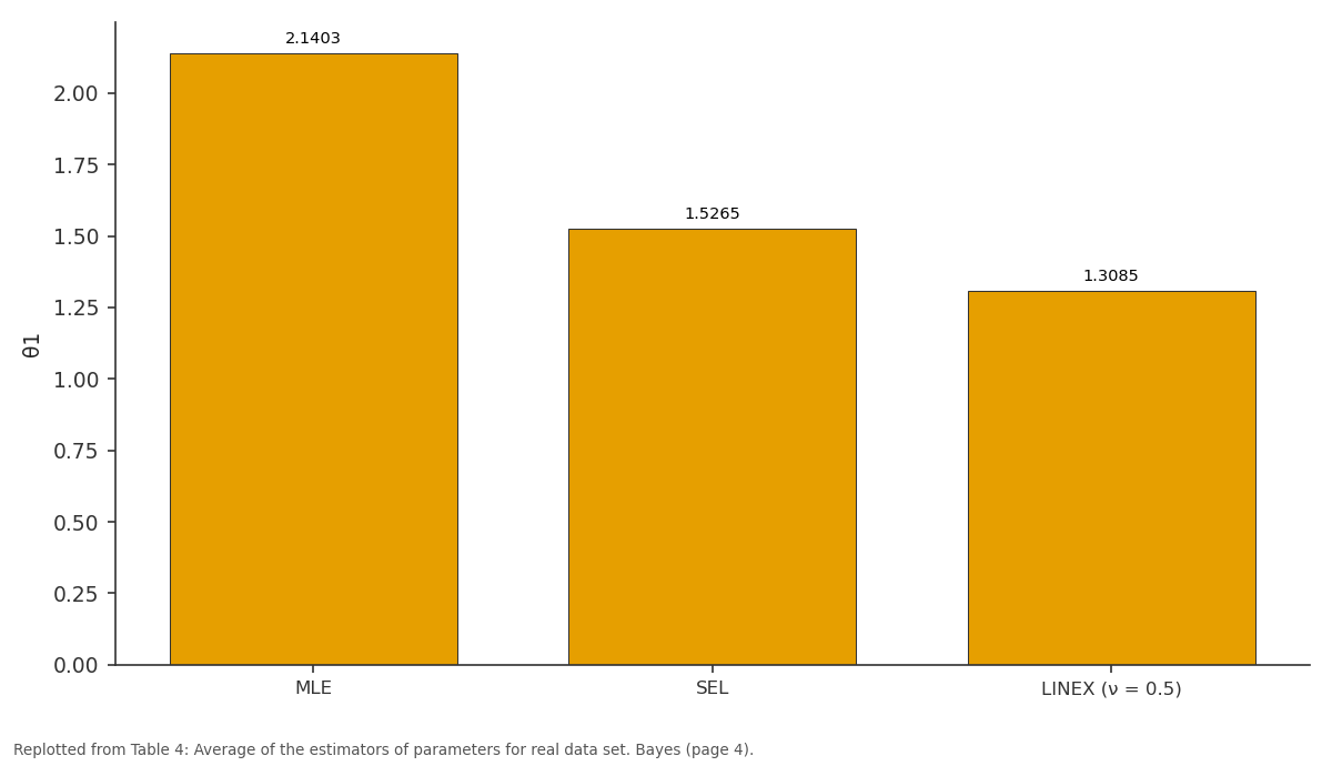
θ1: MLE vs SEL vs LINEX (ν = 0.5)
Replotted from Table 4 (page 4) of the original paper. Every bar is the paper's own table value.
View source evidence ↗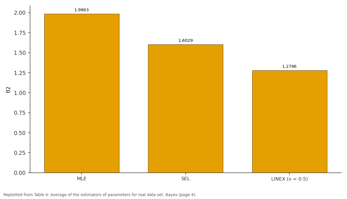
θ2: MLE vs SEL vs LINEX (ν = 0.5)
Replotted from Table 4 (page 4) of the original paper. Every bar is the paper's own table value.
View source evidence ↗Figures & tables
From the original paper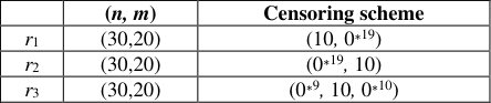 Table 1
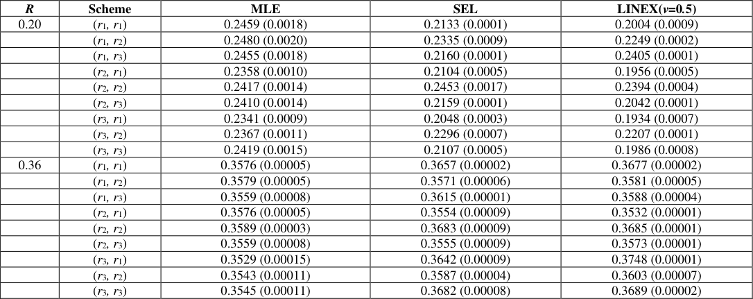 Table 2
 Table 3
 Table 4
Introduction
In the field of reliability and life testing experiments, observing failure times of units put on tests is non-conventional. This may be due to varied restrictions on data collection like cost effectiveness, total time of test, simplicity of experimental set-up and many more. These constraints are manoeuvre by an experimenter which results in censoring of data arising in an experiment. Among various censoring schemes, the type-II progressive censoring scheme has become very popular. It can be explained as follows. Let n items be put in a life time study and m(< n) items be completely observed; At the time of first failure, r1 surviving units are removed from the n-1 remaining items; At the time of the next failure, r 2 items are randomly withdrawn from the nr 1 -2 remaining items; when the nth failure occurs the remaining nmr 1 -. . . -r m-1 items are removed. See Balakrishnan (2007) [2] for more details. There has been continuous interest in the problem of estimating the probability that one random variable exceeds another, that is, R=P (X > Y), where X and Y are independent random variables. The parameter R is referred to as the reliability parameter. This problem arises in the classical stress-strength reliability where one is interested in assessing the proportion of the times the random strength X of a component exceeds the random stress Y to which the component is subjected. If X ≤ Y, then either the component fails or the system that uses the component may malfunction. This problem also arises in situations where X and Y represent lifetimes of two devices and one wants to estimate the probability that one fails before the other. Estimation of the stress-strength parameter has received considerable attention in the statistical literature. Various authors have studied the estimation of R based on complete samples. A comprehensive account of this topic is given by Kots et al. (2003) [7] . Recently, some authors have studied the inferential procedures of R for some lifetime distributions based on progressive type-II censored samples. See, for example, Asgharzadeh et al. (2011) [1] , Rezaei et al. (2015) [10] and Saraçoğu et al. (2015). The aim of this paper is to estimate R = P (Y < X) under progressive type-II censored data on both variables X and Y, when X and Y are independent Poisson-Exponential random variables.
A random variable X is said to have a Poisson-Exponential (PE) distribution if its probability density function (pdf) and cumulative distribution (cdf) is given by Respectively. Here, the parameter θ is a shape parameter and λ is a scale parameter. From now on, PED with the shape parameter θ and scale parameter λ will be denoted by PE(θ, λ).
Maximum Likelihood Estimation of R
Let X ∼ PE(θ1, λ) and Y ∼ PE(θ 2 , λ) be independent random variables with unknown shape parameters θ 1 and θ 2 and common scale parameter λ. The stress-strength parameter, R is ( )
Our interest is in estimating R based on progressive censored samples on both variables. Suppose X = (X 1:m1:n1 , . . . , X m1 :m1 :n1 ) is a progressively type-II censored sample from PE(θ 1 , λ) with censored scheme r 1 and Y = (Y 1:m2 :n2 , . . . , Y m2 :m2 :n2 ) is a progressively type-II censored sample from PE(θ 2 , λ) with censored scheme r 2 , where r i = (r i1 , . . . , r im ) and
For the sake of simplicity, we will write (X 1 , . . . , X m1 ) instead of (X 1:m1:n1 , . . . , Xm1 :m1 :n1 ) and (Y 1 , . . . , Y m2 ) instead of (Y 1:m2:n2 , . . . , Y m2 :m2 :n2 ). The likelihood and log-likelihood function obtained as follows (see Balakrishnan and Aggarwala (2000)) [3] .
The MLEs of parameters can be obtained as the simultaneous solutions of ( ) ( )
To compute the maximum likelihood estimator (MLE) of R, we need to compute the MLEs of θ 1 and θ 2 , say θˆ1 and θˆ2, respectively. The MLE Rˆ of R can then be obtained by substituting θˆi in place of θ i in (2.1), for i = 1, 2. Since, there exists no closed form for above likelihood equations, then we use the Newton-Raphson algorithm to obtain the MLEs of the unknown parameters.
Bayes Estimation of R In this section, we obtain the Bayes estimation of R under assumption that all of the parameters θ 1 , θ 2 and λ are unknown. We assume that θ 1 and θ 2 have the gamma prior, i.e, π(θ 1 ) ∼ Γ(a 1 , b 1 ) and π(θ 2 ) ∼ Γ(a 2 , b 2 ), respectively. Also, we consider a prior Gamma (a 3 , b 3 ) for the scale parameter λ. Moreover, it is assumed that θ 1 , θ 2 and λ are independent. Therefore the joint posterior density of θ 1 , θ 2 and λ is given by ( ) ( )
∫∫∫ x y x y x y
Clearly, the form of the posterior density does not lead to explicit Bayes estimators of the model parameters. For this, we need a simulation technique to compute the Bayes estimator of R. We adopt the importance sampling method to generate samples from the posterior distributions and then compute the Bayes estimators of R under Squared Error (SEL) and LINEX loss function. The posterior distributions of θ 1 , θ 2 and λ can be obtained as follows:
Now consider the following steps to draw samples from the above posterior density.
Step 2: Given λ (k) generate θ 1 (k) from
Step 4: Compute R (k) from by substituting θ (k) and θ (k) in place of θ 1 and θ 1 in (2.1).
Step 5: Repeat steps 2-4, M times. Now the Bayes estimator of R under SEL and LINEX loss functions becomes:
Simulation study
In this section, a Monte Carlo simulation study is conducted to investigate and compare the performance of all estimators presented in this paper. We use the three censoring schemes in Table 1. The performances of the MLEs and the Bayes estimates with respect to the squared error and LINEX loss functions mainly are compared in terms of mean squares errors (MSEs). We consider the hyper parameters as a 1 = b 1 = a 2 = b 2 = 0.0001. The results are reported based on 1000 replications. We obtain the estimates of R by MLE and by using the Bayesian procedure under squared error and LINEX loss function. The results are reported in Table 2. Based on simulation results, we observed that the MSEs of the Bayes estimators are smaller than the MSEs of the MLEs. The (r 1 , r 3 ) has smaller MSE compared to the other schemes.
| R | Scheme | MLE | SEL | LINEX(ν=0.5) |
|---|---|---|---|---|
| 0.20 | (r1, r1) | 0.2459 (0.0018) | 0.2133 (0.0001) | 0.2004 (0.0009) |
| (r1, r2) | 0.2480 (0.0020) | 0.2335 (0.0009) | 0.2249 (0.0002) | |
| (r1, r3) | 0.2455 (0.0018) | 0.2160 (0.0001) | 0.2405 (0.0001) | |
| (r2, r1) | 0.2358 (0.0010) | 0.2104 (0.0005) | 0.1956 (0.0005) | |
| (r2, r2) | 0.2417 (0.0014) | 0.2453 (0.0017) | 0.2394 (0.0004) | |
| (r2, r3) | 0.2410 (0.0014) | 0.2159 (0.0001) | 0.2042 (0.0001) | |
| (r3, r1) | 0.2341 (0.0009) | 0.2048 (0.0003) | 0.1934 (0.0007) | |
| (r3, r2) | 0.2367 (0.0011) | 0.2296 (0.0007) | 0.2207 (0.0001) | |
| (r3, r3) | 0.2419 (0.0015) | 0.2107 (0.0005) | 0.1986 (0.0008) | |
| 0.36 | (r1, r1) | 0.3576 (0.00005) | 0.3657 (0.00002) | 0.3677 (0.00002) |
| (r1, r2) | 0.3579 (0.00005) | 0.3571 (0.00006) | 0.3581 (0.00005) | |
| (r1, r3) | 0.3559 (0.00008) | 0.3615 (0.00001) | 0.3588 (0.00004) | |
| (r2, r1) | 0.3576 (0.00005) | 0.3554 (0.00009) | 0.3532 (0.00001) | |
| (r2, r2) | 0.3589 (0.00003) | 0.3683 (0.00009) | 0.3685 (0.00001) | |
| (r2, r3) | 0.3559 (0.00008) | 0.3555 (0.00009) | 0.3573 (0.00001) | |
| (r3, r1) | 0.3529 (0.00015) | 0.3642 (0.00009) | 0.3748 (0.00001) | |
| (r3, r2) | 0.3543 (0.00011) | 0.3587 (0.00004) | 0.3603 (0.00007) | |
| (r3, r3) | 0.3545 (0.00011) | 0.3682 (0.00008) | 0.3689 (0.00002) |
Table text extracted from the original PDF; superscript letters are shown inline. The original table image is below.
View original table image
| — | (n, m) | Censoring scheme |
|---|---|---|
| r1 | (30,20) | (10, 0∗19) |
| r2 | (30,20) | (0∗19, 10) |
| r3 | (30,20) | (0∗9, 10, 0∗10) |
Table text extracted from the original PDF; superscript letters are shown inline. The original table image is below.
View original table image
Numerical example
Here, we consider a data analysis for the data set reported by Pepi (1994) [9] . The data set describes the all-glass airplane window design that measure polished window strength. The data sets are as follows:
25. Next we obtain the values of unknown parameters to compute the the values of R. To compute the Bayes estimate, since we do not have any prior information, we assumed that a1 = b 1 = a 2 = b 2 = 0.0001. The MLE and Bayes estimators of R under SEL and LINEX loss functions become 0.1986 and 0.07075, 0.0414, respectively.
Conclusion
In this paper, we consider the estimation of the stress-strength parameter of Poisson-Exponential distribution. It is assumed that the two populations have the same scale parameters, but different shape parameters. It is observed that the maximum likelihood estimators of the unknown parameters cannot be obtained in closed form. For this, we use the iterative method as the Newton-Raphson (NR) algorithm. Further we obtain the Bayes estimators of R under squared error and LINEX loss function. Based on simulation results it is observed that Bayes estimators based on LINEX loss function has more low risk than SEL function.
Figures and tables from the paper
| — | (n, m) | Censoring scheme |
|---|---|---|
| r1 | (10,5) | (5, 0∗4) |
| r2 | (12,5) | (7, 0∗4) |
Table text extracted from the original PDF; superscript letters are shown inline. The original table image is below.
View original table image
| Parameter | MLE | SEL | LINEX (ν = 0.5) |
|---|---|---|---|
| θ1 | 2.1403 | 1.5265 | 1.3085 |
| θ2 | 1.9863 | 1.6029 | 1.2796 |
| λ | 0.0179 | 0.0185 | 0.0167 |
Table text extracted from the original PDF; superscript letters are shown inline. The original table image is below.
View original table image
References
10 in the original paper- Asgharzadeh A, Valiollahi R, Raqab MZ. Stress-strength reliability of Weibull distribution based on progressively censored samples, SORT. 2011;35:103-124.
- Balakrishnan N. Progressive censoring methodology: an appraisal (with discussions). TEST. 2007;16:211-296.
- Diebolt J, Celeux G. Asymptotic properties of a stochastic EM algorithm for estimating mixing proportions. Stochastic Models. 1990;9:599-613.
- Gelfand AE, Smith AFM. Sampling-based approaches to calculating marginal densities, Journal of American Statistical Assocasion. 1990;85:398-409.
- Hastings WK. Monte Carlo sampling methods using Markov chains and their applications, Biometrika. 1970;57:97-109.
- Pepi JW. Failsafe design of an all BK-7 glass aircraft window. SPIE Proc. 1994;2286:431-443.
- Rezaei S, Alizadeh Noughabi R, Nadarajah S. Estimation of stress-strength reliability for the generalized Pareto distribution based on progressively censored samples. Journal of Annals Data Sciences, 2015. Doi: 10.1007/s40745-015-0033-0.
- Saraçoglu B, Kınacı I, Kundu D. On estimation of R = P (Y < X) for exponential dis-tribution under progressive type-II censoring. Journal of Statistical Computation and Simulation. 2012;85:729-744.
- Wang FK, Cheng Y. EM algorithm for estimating the Burr XII parameters with multiple censored data. Quality and Reliab Engineering International. 2010;26:615-630.
- Wei GC, Tanner MA. A Monte Carlo implementation of the EM algorithm and the poor man's data augmentation algorithms. Journal of American Statistical Assocasion. 1990;85:699-704.