
Research article · 2022 · Full text
International Journal of Statistics and Applied MathematicsShock model approach to change points with ERLANG threshold
Volume 7(5) · Pages 142–145 · DOI: 10.22271/maths.2022.v7.i5b.914 ↗
Research areasReliability and Maintenance OptimizationRisk and Safety AnalysisSoftware Reliability and Analysis Research
Abstract
Author-writtenCumulative damage process is related to shock models in reliability theory. The threshold or withstanding capacity of the system can be considered to be any one of the constant level, cumulative shock random threshold level, maximum shock random threshold etc. In this paper, cumulative shock random threshold level is considered wherein a system undergoes a shock and encounters random amount of damage but the system survives with the damages. Successive shocks at random epochs lead to the cumulative damages and when the cumulative damage crosses the threshold level of the system, the system fails. Assuming threshold level undergoes a change in the form of distribution after the change points are taken to be ERLANG random variable, the distribution function for the threshold level is obtained by taking exponential distribution as the threshold levels are before, in between and after the change points respectively. Using this distribution function for the threshold level, the expected time to the breakdown of the system and its variance are obtained by using shock model and cumulative damage process approach.
Summary
Source-checkedPlain-language reading of the full paper, prepared with AI and checked against the text. Each point links to the authors' own words.
Why it matters
- The study is based on reliability theory, specifically using shock models and cumulative damage processes. View evidence ↗
- In these models, a system fails when the accumulation of random damages from successive shocks exceeds a specific threshold level. View evidence ↗
- The threshold, or the system's capacity to withstand damage, can be modeled as a constant or as various types of random variables. View evidence ↗
The question
- The research aims to determine the expected time to system breakdown and its variance using a specific distribution function for the threshold level. View evidence ↗
What they did
- The model assumes the threshold level follows an exponential distribution before, between, and after change points, with the change points themselves being Erlang random variables. View evidence ↗
- The model assumes that the processes generating manpower wastage and the interarrival times between decision epochs are mutually independent. View evidence ↗
- Manpower wastage at each decision epoch is represented by a random variable Xi with a specific probability density function (PDF) and cumulative distribution function (CDF). View evidence ↗
What they found
- As the parameter d increases from 1 to 10, the expected time to recruitment E(T) decreases from 3 to 0.3. View evidence ↗
- When the threshold parameter increases from 0.5 to 2.5, the expected time to recruitment E(T) decreases from 9.01 to 3.74. View evidence ↗
- As the parameter τ1 increases from 0.5 to 2.5, the expected time to recruitment E(T) increases from 4.51 to 34.20. View evidence ↗
What it means
- The authors conclude that increasing the damage magnitude parameter d increases the expected time to recruitment because the average level of depletion decreases. View evidence ↗
- The authors state that increasing the threshold parameter leads to a decrease in E(T) because the mean value of the exponentially distributed threshold decreases. View evidence ↗
- The authors conclude that increasing the parameter τ1 after the first change point increases E(T), as the threshold follows an Erlang 2 distribution after the truncation point. View evidence ↗
Visual summary
3 visualsIllustrations explain the paper; charts are replotted from the paper's own table values.

Cumulative Damage Process
AI-generated conceptual illustration (a mechanical steel gear system). It explains the idea and does not show study data.
View source evidence ↗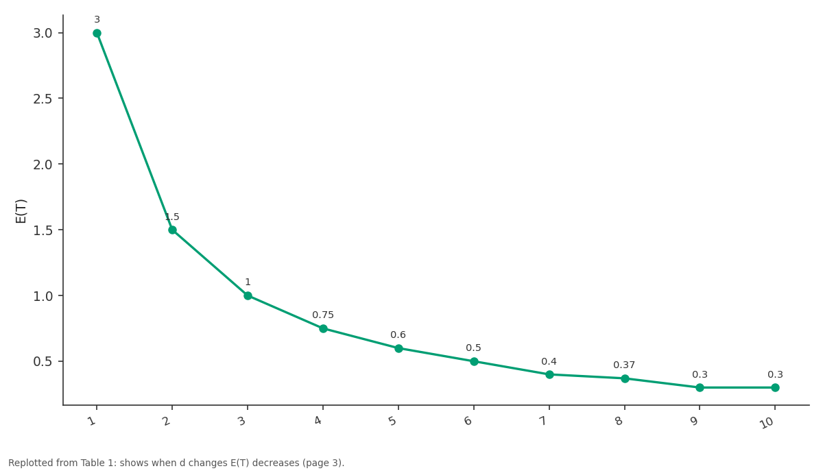
E(T): 1 vs 2 vs 3 vs 4 vs 5
Replotted from Table 1 (page 3) of the original paper. Every bar is the paper's own table value.
View source evidence ↗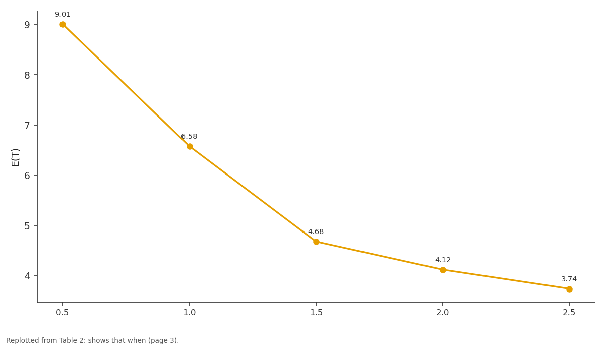
E(T): 0.5 vs 1.0 vs 1.5 vs 2.0 vs 2.5
Replotted from Table 2 (page 3) of the original paper. Every bar is the paper's own table value.
View source evidence ↗Figures & tables
From the original paper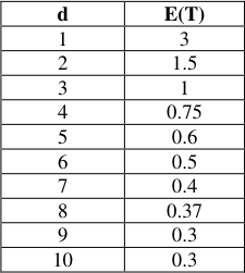 Table 1
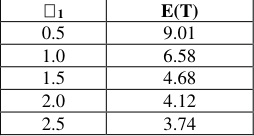 Table 2
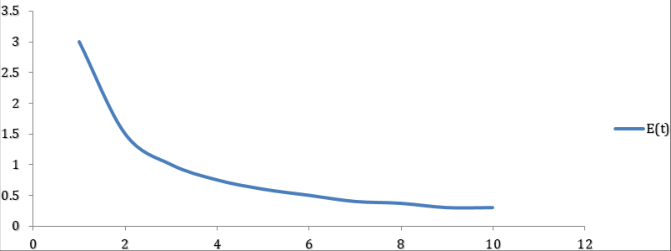 Figure 1
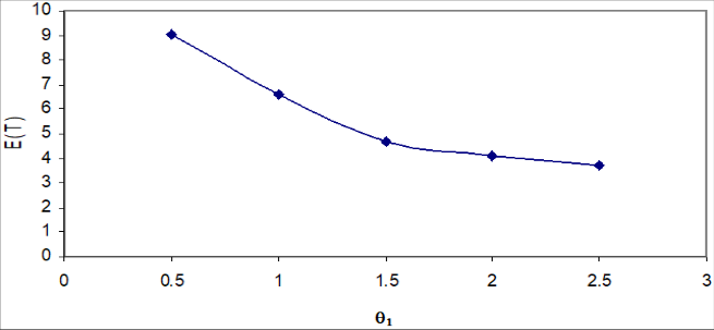 Figure 2
 Table 3
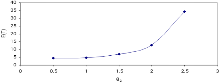 Figure 3
Introduction
In deriving the expression for the expected time to recruitment after change points using exponential distribution of E (T) and its variance V (T) is discussed in chapter IV, if the manpower takes place at the decision epochs. Under the assumption that threshold random variable under goes a changes of distribution from exponential and ERLANG after two change points. In doing so it has been assumed that the inter arrival times between the decisions epochs are identically independently distributed (I.I.D). In this chapter it is assumed that the random variables denoting the inter arrival times between decision epoch of Mean and Variance are derived.
Numerical illustrations are also provided. 2. Assumptions of the model 1. Wastage of manpower occurs at the policy decision epochs. 2. The threshold is a random variable whose distribution undergoes a change after a change point. 3.
The process that generates the wastages and the interarrival times are mutually independent. 4. The breakdown of the activities occurs as and when the cumulative wastage crosses a threes Maths 2022; 7(5): 142-145 https://www.mathsjournal.com R Subathira Department of Statistics, Annamalai University, Annamalai Nagar, Tamil Nadu, India N Vijayshankar Assistant Professor, Department of Statistics, Annamalai University, Annamalai Nagar, Tamil Nadu, India R Subathira Department of Statistics, Annamalai University, Annamalai Nagar, Tamil Nadu, India hold level. This in other words is the time to recruitment. 3. Notations Xi = A random variable denoting the amount of manpower wastage of the ith decision epoch, i = 1, 2, k with P.D.F g (x) and C.F.F G (x).
Y = A random variable denoting the threshold with P.D.F. h (y) and C.F.F H (y). Ui = A random variable denoting the interarrival times between depletions of manpower, i = 1, 2, k with P.D.F. f (.) and C.F.F F (.) T = A random variable denoting the time to recruitment with P.D.F and L (.) Gk (x), Fk (x) = are the k convolution of G (.) and F (.) respectively L* (s) = Laplace transform of and L (.) respectively https://www.mathsjournal.com y 1 , y if e 1 1 y 1 2 1 1 , y if e y e 2 1 2 2 1 y h y 2 3 i e y 2 2 3 1 2 2 1 1 y if e e , 1 2 1 2 2 It is represented by k i ) ( ) ( dx x H x g Y x P k i 0 1 (6.1) k i 1 ) ( dx x H x g Y x P k i 0 1 k k x y x P t F t F t S 1 ) ( i k 1 0 i (6.2) k k k 1 2 1 1 2 1 d e g y x P i 2 * 2 * g e g d 2 2 1 * k 2 3 2 1 2 1 d e e 3 * g d (6.3) 3 3 k k 2 3 2 1 2 1 2 3 2 1 2 1 d e e g e e 3 * g d 3 3 1 2 2 3 * k 2 3 2 1 2 1 g e e 3 * 1 2 2 Y X P t F t F t S ] [ )] ( ) ( [ ) ( i i k k k 0 2 3 2 1 2 1 1 2 1 1 2 1 d e g )] ( [ )] ( [ )] ( [ )] ( K k K k K k K k 3 * d e e g e g d g d 2 2 ) ( 1 * 3 3 ) ( ) ( 3 * ) ( 2 * 2 3 2 1 2 1 2 3 2 1 2 1 2 3 2 1 2 1 d e e g e e ] ( )[ ( )] ( [ ) ( )] ( [ k K k K k 3 * 1 2 2 ) ( ) ( 3 * g e e g d 3 3 1 2 2 ) ( ) ( 3 * 3 ) ( ) ( (6.4) 4. On simplification 1 2 1 1 2 1 )] ( [ )] ( ) ( [ )] ( [ )] ( ) ( [ )] ( )] ( ) ( [ d e t F t F g t F t F i k k 3 * ) ( g e t F t F g d i k k K k k 0 0 1 * i k k K k k 0 2 * K k k 2 2 ) ( 2 3 2 1 2 1 2 3 2 1 2 1 )] ( [ )] ( ) ( [ )] ( [ )] ( ) ( [ d e e t F t F i k k 3 * 3 ) ( ) ( g e e t F t F g d i k k K k k 0 0 3 * K k k 3 3 ) ( ) ( 2 3 2 1 2 1 2 3 2 1 2 1 ] ( )[ ( )] ( ) ( [ )] ( [ ) ( )] ( ) ( [ d e e t F t F i k k 3 * 1 2 2 ) ( ) ( g e e t F t F g d i k k K k k 0 0 3 * k k k 3 3 1 2 2 ) ( ) ( Using the equation (6.4) then, https://www.mathsjournal.com t S t H ) ( 1 ) ( 1 2 1 )] ( [ )] ( ]) ( ) ( [ )) ( 1( 1 1 d t F e g t F g 1 * 1 * k K k i k k ) ( 2 1 2 * g d k 1 2 2 0 1 2 1 1 2 1 d t F e )] ( )[ ( [ )] ( 1( 1[ )] ( [ )] ( ) ( 2 K k k k K k i k 1 3 * 2 * ) ( 2 * g t F g e g d k 1 2 0 2 3 2 1 2 1 d t F e e )] ( [ ) ( k k k 3 * g d 3 0 3 ) ( ) ( k 2 3 2 2 2 1 d t F e e ) ( ) ( 1 ) ( ) ( 3 k 3 * g d 3 0 k k 1 2 3 2 1 2 1 2 3 2 2 2 1 g e e g t F g e e ]) ( [ ) ( ]) ( )[ ( )] ( 1( 1[ 3 * 3 ) ( ) ( K k 3 * 1 2 3 ) ( ) ( 1 k 1 k 1 𝑑𝐻∗ (𝑠) (6.5) 𝐸(𝑇) = 𝑑(𝑠) /s=0 (𝜔+ 𝜃1) 𝐸(𝑇) = ( ) −(𝑒− (𝜃1 – 𝜃2)𝜏1 ) ( 𝑑𝜔2 𝑑𝜃1 (𝑑𝜃2)2) −(𝑒−(𝜃1 – 𝜃2)𝜏1 −(𝜃2 – 𝜃3)𝜏2 ) ( 𝑑𝜔2 (𝑑𝜃3)2) −(𝑒−(𝜃1 – 𝜃2)𝜏1−(𝜃2 – 𝜃3)𝜏2 )(𝜃2 (𝜏2 −𝜏1)) ( 𝑑𝜔2 (𝑑𝜃3)2) 5. Mathematical Illustration Table 2: shows that when increases then E(T) decreases.
| 1 | E(T) |
|---|---|
| 0.5 | 9.01 |
| 1.0 | 6.58 |
| 1.5 | 4.68 |
| 2.0 | 4.12 |
| 2.5 | 3.74 |
Table text extracted from the original PDF; superscript letters are shown inline. The original table image is below.
View original table image
Table 1: shows when d changes E(T) decreases d E(T) 1 3 2 1.5 3 1 4 0.75 5 0.6 6 0.5 7 0.4 8 0.37 9 0.3 10 0.3 1 E(T) 0.5 9.01 1.0 6.58 1.5 4.68 2.0 4.12 2.5 3.74 Fig 1: E (T) Fig 2: https://www.mathsjournal.com Table 3: Variation in E (T) for Changes τ1 τ1 E(T) 0.5 4.51 1.0 4.68 1.5 7.07 2.0 12.92 2.5 34.20 Fig 3:
| τ1 | E(T) |
|---|---|
| 0.5 | 4.51 |
| 1.0 | 4.68 |
| 1.5 | 7.07 |
| 2.0 | 12.92 |
| 2.5 | 34.20 |
Table text extracted from the original PDF; superscript letters are shown inline. The original table image is below.
View original table image
| d | E(T) |
|---|---|
| 1 | 3 |
| 2 | 1.5 |
| 3 | 1 |
| 4 | 0.75 |
| 5 | 0.6 |
| 6 | 0.5 |
| 7 | 0.4 |
| 8 | 0.37 |
| 9 | 0.3 |
| 10 | 0.3 |
Table text extracted from the original PDF; superscript letters are shown inline. The original table image is below.
View original table image
Conclusion
The following conclusions can be drawn on the basis of the numerical illustration taken up in this model. Case (i): As the value of d which is the parameter of the random variable denoting the magnitude the damages namely X increases then E (T) increases. This is due to the fact that the average level of depletion decreases and hence E(T) increases. Case (ii): As the value 1 which is the parameter of the random variable denoting the threshold increases, E(T) decreases.
This is due to the fact that the threshold random variable is exponentially distributed and hence its mean value decreases when the parameter increases. Hence E(T) becomes smaller Case (ii): As the value of τ1 which is the parameter of the threshold after the first change point increases then E(T) also increases. This is due to the fact that in this model the threshold follows ERLANG 2 distribution after the truncation point. The threshold level becomes smaller, as τ1 increases.
Only after the truncation point but prior to the truncation point it is higher, so due to the combined value of threshold E(T) increases.
References
9 in the original paper- Barthlomew DJ, Forbes A. Statistical techniques for manpower planning, John Wiely Sons; c1979.
- Esary JD, Marshall AW, Proschan F. Shock models and Wear Processes, The Annals of Probability. 1973;1(4):627-649.
- Hameed AMS, Proschan F. Shock models with underlying birth process, Journal of Applied Probability. 1975;12:18-28.
- Sathiyamoorthi R, Elangovn R. Shock model approach to determine the expected time for recruitment, Journal of Decision and Mathematical Sciences. 1998;3(1-3):67-78.
- Sathiyamoorthy R, Parthasarathy S. On the expected time to recruitment when threshold distribution has SCBZ property,
- Grinold RC. Manpower planning with Uncertain Recruitments, Operations Research. 1976;24:387-400.
- Grinold RC, Marshall KT. Manpower Planning Models, North Holland, New York; c1977.
- Gurland J. Distribution of Maximum of the Arithmetic Mean of Correlated Random Variables, Ann. Math. Statustm. 1955;26:294-300.
- Hayne NJ, Marshall KT. Two Characteristic Markov- Type Manpower Flow Models, Naval Research Logistics Quarterly. 1974;24:235-256.