
Research article · 2022 · Full text
International Journal of Statistics and Applied MathematicsA stochastic approach using Garima distribution
Volume 7(6) · Pages 157–163 · DOI: 10.22271/maths.2022.v7.i6b.912 ↗
Research areasStatistical Distribution Estimation and ApplicationsProbabilistic and Robust Engineering DesignAdvanced Statistical Methods and Models
Abstract
Author-writtenIn this article we propose a power Garima distribution which includes Garima distribution as particular case. Its statistical properties including behavior of its probability density function for varying values of parameters, moments, hazard rate function and mean residual life function has been discussed. The estimation of the parameters of the distribution has been discussed using maximum likelihood estimation.
Summary
Source-checkedPlain-language reading of the full paper, prepared with AI and checked against the text. Each point links to the authors' own words.
Why it matters
- The Garima distribution is a continuous probability distribution designed to model data from real-life time databases. View evidence ↗
The question
- The authors aim to propose a 'power Garima distribution' (PGD), which serves as a generalization that includes the original Garima distribution as a special case. View evidence ↗
What they did
- The study analyzes the PGD by deriving its probability density function (pdf), moments, hazard rate function, and mean residual life function. View evidence ↗
- Maximum likelihood estimation (MLE) is employed to determine the parameters of the proposed distribution. View evidence ↗
- The parameter estimation is based on a random sample of size n drawn from the power Garima distribution. View evidence ↗
- The authors utilize Fisher's Information matrix to analyze the properties of the maximum likelihood estimators. View evidence ↗
What they found
- The authors demonstrate the utility of the power Garima distribution through a numerical example. View evidence ↗
- The power Garima distribution provides a better fit for the tested data compared to the Garima, exponential, and Lindley distributions. View evidence ↗
What it means
- The authors conclude that they have successfully developed a new generalization of the power Garima distribution using a stochastic approach. View evidence ↗
Visual summary
1 visualsIllustrations explain the paper; they do not show study data.

Distribution Hierarchy
AI-generated conceptual illustration (Abstract geometric spheres representing mathematical probability distributions). It explains the idea and does not show study data.
View source evidence ↗Figures & tables
From the original paper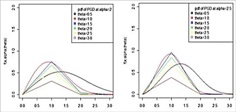 Figure 1
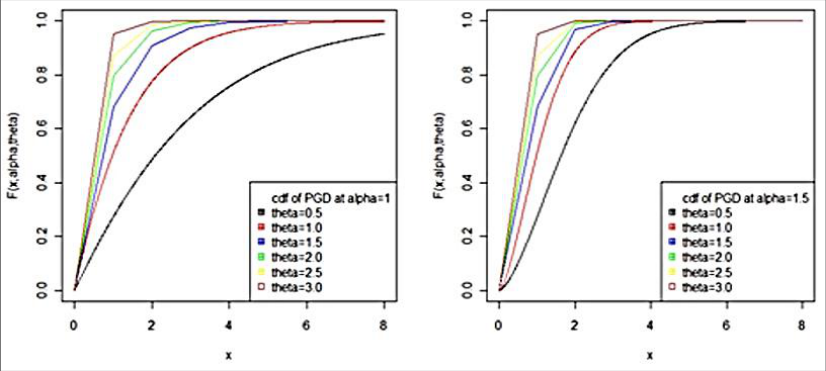 Figure 1
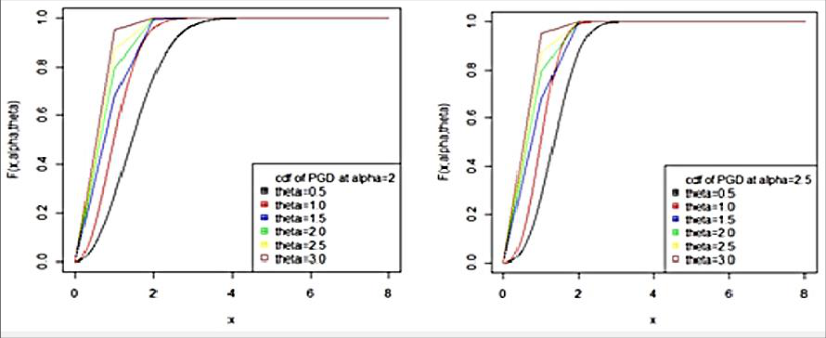 Figure 2
Introduction
In this research paper a continuous distribution named “Garima distribution” has been suggested for modelling data from real life time database. The important properties including its shape, moments, skewness, kurtosis, hazard rate function, mean residual life function, stochastic ordering, mean deviations have been discussed. The condition under which Garima distribution is over dispersed, uniform dispersed, and under-dispersed are presented along with other one parameter continuous distributions. The estimation of its parameter has been discussed using maximum likelihood estimation and method of moments.
The application of the proposed distribution has been explained using a numerical example. Power Garima Distribution (PGD) The probability density function of power Garima distribution (PGD) is given by x θx x θx x; f ( ) ( ) ) 1.7 ( 0 ,0 ,0 ; e 1 1 2 , − − + + + = and the cumulative distribution function of power Garima distribution is given by Maths 2022; 7(6): 157-163 https://www.mathsjournal.com R Subathira Department of Statistics, Annamalai University, Annamalai Nagar, Tamil Nadu, India N Vijayshankar Assistant Professor, Department of Statistics, Annamalai University, Annamalai Nagar, Tamil Nadu, India R. Subathira Department of Statistics, Annamalai University, Annamalai Nagar, Tamil Nadu, India https://www.mathsjournal.com Fig 1: Graphs of pdf of PGD for varying values Fig 2: Graphs of the cdf of PGD for varying values of the Reliability Measures Survival function The survival function is also known as reliability function. it can be computed as complement of the cumulative distribution function. The survival function or the reliability function of power Garima distribution is given by ) , ; ( 1 ) ( x lF x S − = x S ,)1 2 ( ,)1 ( ,)1 ( 1 1 ) ( )1 2 ( )1 ( )1 ( θx θx θx − = + + + + + + + + + + θ https://www.mathsjournal.com Hazard function The hazard function is also known as hazard rate, instantaneous failure rate or force of mortality and is given by x lf x h ) , ; ( ) ( = x S ) ( + 1 ) 1( − + + θx e θx x h(x) = , )1 2 ( , )1 ( , )1 ( )1 2 ( )1 ( )1 ( θx θx θx + + + + + − + + + + + Reliability function of Power Garima Distribution Hazard function of power Garima Distribution Structural Properties Here, I discuss some statistical properties of power Garima distribution. https://www.mathsjournal.com Moments Let X represents the random variable of power Garima distribution with parameters θ and α, then the rth order moment E(X r) of power Garima distribution is obtained as = = ) , ; ( ) ( ' dx x lf r x r X E r 0 1 ) 1( − + + + + = dx θx e θx r x 0 )1 2 ( )1 ( )1 ( + + + + + θ + 1 = dx θx e θx r x ) 1( )1 2 ( )1 ( )1 ( 0 − + + + + + + + + θ + 1 2 = dx θx e r x dx θx e r x dx θx e r x + − + + − + + 0 )1 2 ( )1 ( )1 ( ) 3.7 ( 0 0 − + + + + + θ 1 ) ( Put t x t x = = dt dt dx dt dx x 1 1 1 Also − = − = = − x t After simplification, equation (7.3) becomes )1 2 ( )1 ( )1 ( r r r ) ( ' + + + + + + + + = = r X E r r ) 4.7 ( )1 2 ( )1 ( )1 ( + + + + + Substitute r = 1 and 2 in equation (7.4), we get mean and the second moment of power Garima distribution. ) 2 2 ( ) 2 ( ) 2 ( + + + + + = = ) ( '1 X E )1 2 ( )1 ( )1 ( 1 + + + + + ) 3 2 ( ) 3 ( ) 3 ( + + + + + = = ) 2 ( ' 2 X E )1 2 ( )1 ( )1 ( 2 + + + + + https://www.mathsjournal.com 2 ) 3 2 ( ) 3 ( ) 3 ( ) 2 2 ( ) 2 ( ) 2 ( + + + + + = ) 2 ( Variance )1 2 ( )1 ( )1 ( 2 )1 2 ( )1 ( )1 ( 1 + + + + + − + + + + + θ θ + + + + + Moment Generating Function Moment generating function is the expected function of the random variable. we begin with the well-known definition of the moment generating function given by ( ) dx (x; lf tx e tx e E t X M ) , 0 ) ( = = 2 1 dx x lf (tx) tx ) , ; ( ... !2 0 + + + = l j j dx x f x j t = = ) , ; ( ! j 0 0 j t = = 0 ' ! j j j )1 2 ( )1 ( )1 ( j j j j t + + + + + + + + = = 0 ! j j j )1 2 ( )1 ( )1 ( + + + + + )1 2 ( )1 ( )1 ( 1 ) ( j t t X M j = = + + + + + + + + + + + + + ! )1 2 ( )1 ( )1 ( j j j j j 0 Characteristic function Characteristic function is defined as the function of any real-valued random variable completely defines the probability distribution of a random variable.
The characteristic function of power Garima distribution is given by ) ( ) ( it X M t x = )1 2 ( )1 ( )1 ( 1 ) ( j it it X M j j j j )1 2 ( )1 ( )1 ( j = = + + + + + + + + + + + + + 0 j ! Maximum Likelihood Estimation and Fisher’s Information matrix In this section, we will discuss about the maximum likelihood estimation of power Garima distribution for estimating its parameters and also Fisher’s Information matrix have been discussed. Let x1, x2,…,xn be a random sample of size n from the power Garima distribution, then the likelihood function can be written as n ) , ; ( ) ( x lf x L = = i 1 https://www.mathsjournal.com + 1 1 − + + n i θx e i θx ix x L ) ( = 1 )1 2 ( )1 ( )1 ( i θ = + + + + + n + 1 n x L ) ( ( ) i θx e i θx ix 1 )1 2 ( )1 ( )1 ( i = 1 = − + + + + + + + + 1 n n x L ) ( ( ) i θx e i θx ix n i = 1 = 1 )1 2 ( )1 ( )1 ( − + + + + + + + The log likelihood function is given by n log )1 2 ( )1 ( )1 ( log log 1 log = − + + = i ix i θx n (7.5) 1 1 ) 1 log( 1 i = i ix n n L + + + + + + + − + = n The maximum likelihood estimates of θ and α can be obtained by differentiating equation (7.5) with respect to θ and α and must satisfy the following normal equations 1 ix )1 ( 1 log = )1 2 ( )1 ( )1 ( i = − i ix n + − + = n = + + 0 1 1 1 θ n n L + + + + + + + i θx log ix i θx n 1 = + + + + + + − − = i ix ix n 0 1 log )1 2 ( )1 ( )1 ( 3 log = = − = + + + i ix n n L log 1 1 i i θx n Where ψ (.) is the digamma function. To obtain the confidence interval we use the asymptotic normality
Results
We have that if ( ) ( ) follows as
Result
the state can we , , of MLE the denotes ˆ ,ˆ ˆ = = ( )) ( ,0 ) ˆ ( 1 2 − → − I N n by given is matrix n informatio s Fisher' is ) ( Where I 2 2 log log L E L E 2 1 ) ( − = 2 2 n I log log L E L E 2 Where https://www.mathsjournal.com 2 2 2 2 1 x n n L E + − 2 2 2 2 n )1 ( 1 ) ( log = 1 )1 2 ( )1 ( )1 ( + + + − = 1 + + i θx ( ) ( ) i i + + + + + 2 2 2 n n L E 2 2 3 )1 2 ( )1 ( )1 ( ' ) ( 3 log + + + + + − = 2 2 n n 2 log ) (log 1 x θx x θx θx − + + + i i 2 ( ) − = − 1 i 1 i i i i i x x θx log 1 + + ( ) ( ) ( ) i i 2 2 )1 ( log log n L E L E )1 2 ( )1 ( )1 ( = + − = + + + + + n n 1 log log 1 x x θx x x θx + − + + + i i 2 − = = 1 1 i i i i i i i x x θx log 1 + + ( ) ( ) ( ) i i we unknown, being Since function. diagamma of derivative order first the is (.)' where . and for interval confidence asymptotic obtain to used be can this and )ˆ ( by ) ( estimate 1 1 − − I I
Conclusion
In this paper, we have discussed a new generalization of power Garima distribution using stochastic approach. The different mathematical and statistical properties of the newly introduced distribution have been discussed. The maximum likelihood estimator is also used for estimating the parameters of the proposed distribution and also the fisher’s information matrix have been discussed. Finally, the application of power Garima distribution fits better than the Garima, exponential and lindley distributions.
References
8 in the original paper- Shanker R, Shukla KK. Size-biased Poisson-Garima Distribution with Applications. Biometrics and Biostatistics International Journal. 2017a;6(3):1-6.
- Shanker R, Shukla KK. Zero-Truncated Poisson-Garima Distribution with Applications. Biometrics and Biostatistics Open access Journal. 2017b;3(1):1-6.
- Ghitany ME, Al Mutairi DK, Balakrishnan N, Al-Enezi LJ. Power Lindley distribution and Associated Inference, Computational Statistics and Data Analysis. 2013;64:20-33.
- Lindley DV. Fiducial distributions and Bayes’ Theorem, Journal of Royal Statistical Society. Series B. 1958;20:102-107.
- Shanker R, Hagos F, Sujatha S. On Modeling of Lifetimes data using Exponential and Lindley distributions. Biometrics & Biostatistics International Journal. 2015;2(5):1-9.
- Smith RL, Naylor JC. A comparison of Maximum likelihood and Bayesian estimators for the three parameter Weibull distribution. Applied Statistics. 1987;36:358-369.
- Berhane A. Discretization of some continuous distribution and Their Applications, Master thesis submitted to Department of Statistics, College of Science, Eritrea Institute of Technology, Asmara, Eritrea, 2018.
- Weibull W. A statistical distribution of wide applicability. Journal of Applied Mathematics. 1951;18:293-297.