
Research article · 2022 · Full text
International Journal of Statistics and Applied MathematicsSome properties and applications of half Cauchy extended exponential distribution
Volume 7(4) · Pages 226–235 · DOI: 10.22271/maths.2022.v7.i4c.866 ↗
Research areasStatistical Distribution Estimation and ApplicationsReliability and Maintenance OptimizationProbabilistic and Robust Engineering Design
Abstract
Author-writtenIn this article, we have introduced a new probability distribution having three parameters using half Cauchy family of distribution named half Cauchy extended exponential distribution. The statistical properties and characteristics of the proposed distribution like the hazard rate function (HRF), cumulative hazard function, and the probability density function (PDF), and the cumulative distribution function (CDF), quantile function and the skewness, kurtosis are provided. The parameters of the proposed distribution are estimated using the Cramer-Von-Mises (CVM) least-square estimation (LSE), and maximum likelihood estimators (MLE) methods. A real data set is analyzed to test the goodness-of-fit of the proposed distribution. It is found that the half Cauchy extended exponential distribution performed well as compared to some competing distributions.
Summary
Source-checkedPlain-language reading of the full paper, prepared with AI and checked against the text. Each point links to the authors' own words.
Why it matters
- The exponential distribution is a fundamental tool in applied statistics for modeling reliability and survival data. View evidence ↗
- The half-Cauchy distribution is useful for predicting frequent long-distance spreading events due to its strong tail. View evidence ↗
The question
- The authors aim to introduce and analyze a new three-parameter probability distribution called the half Cauchy extended exponential (HCEE) distribution. View evidence ↗
What they did
- The study derives key statistical properties for the HCEE distribution, including its PDF, CDF, hazard rate, quantile function, skewness, and kurtosis. View evidence ↗
- Three methods are used to estimate the distribution's parameters: Maximum Likelihood Estimation (MLE), Least-Square Estimation (LSE), and Cramer-Von-Mises (CVM) estimation. View evidence ↗
- The model is tested using a real dataset of 101 observations regarding the fatigue life of 6061-T6 aluminum coupons. View evidence ↗
What they found
- Using MLE on the aluminum coupon dataset, the estimated parameters were 𝛽̂=29.6600, 𝜆̂=1018.6973, and 𝜃̂=1.8073, with a log-likelihood of -458.5402. View evidence ↗
- The HCEE distribution showed a better fit than competing models, exhibiting the minimum test statistics and higher p-values (e.g., KS p-value of 0.7999). View evidence ↗
- Comparing information criteria, HCEE achieved a lower AIC (923.0805) and BIC (930.9258) than the Exponentiated Weibull (EW) distribution (AIC 923.5201, BIC 931.3654). View evidence ↗
- The authors found that Maximum Likelihood Estimators (MLE) performed relatively better than the LSE and CVM estimation methods. View evidence ↗
- The PDF of the HCEE distribution is flexible, capable of taking various shapes such as right-skewed or increasing-decreasing. View evidence ↗
What it means
- The authors conclude that the HCEE distribution is highly flexible and suitable for modeling real-life data compared to other fitted distributions. View evidence ↗
Visual summary
2 visualsIllustrations explain the paper; charts are replotted from the paper's own table values.
HCEE Distribution Framework
AI-generated conceptual illustration (Mathematical probability distribution curves). It explains the idea and does not show study data.
View source evidence ↗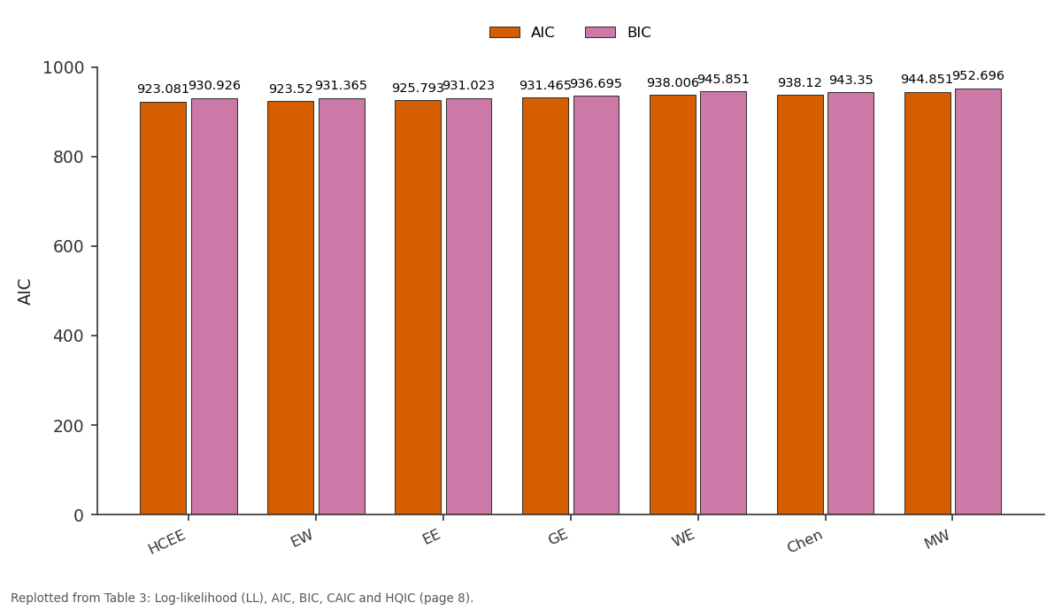
AIC and BIC: HCEE vs EW vs EE vs GE vs WE
Replotted from Table 3 (page 8) of the original paper. Every bar is the paper's own table value.
View source evidence ↗Figures & tables
From the original paper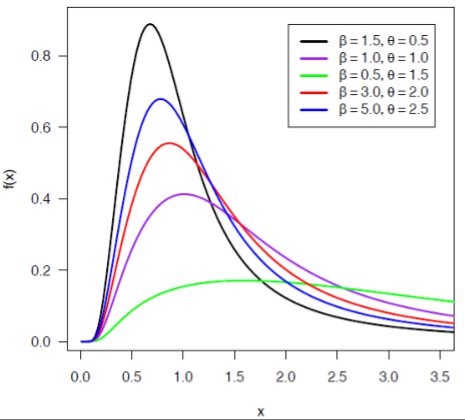 Figure 1
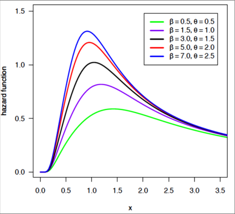 Figure 1
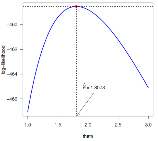 Figure 2
 Table 1
 Table 2
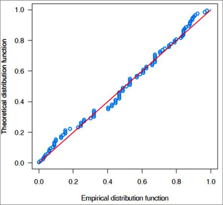 Figure 3
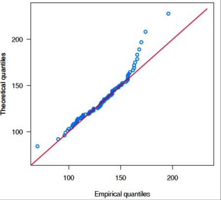 Figure 3
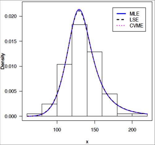 Figure 4
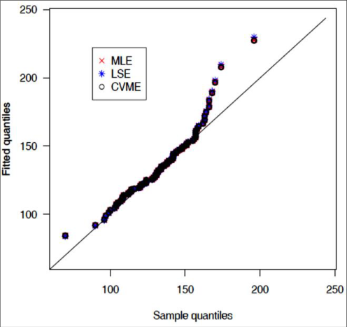 Figure 4
 Table 3
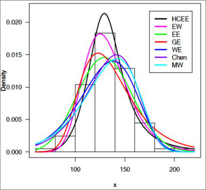 Figure 5
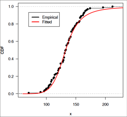 Figure 5
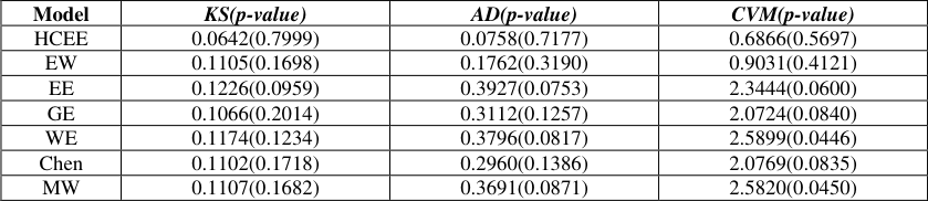 Table 4
Introduction
The exponential distribution (ED) plays a significant role in the modeling of survival and reliability data in applied statistics and probability theory. It has the memoryless property and is a particular case of the geometric and gamma distributions. In addition it can be applied for the study of the Poisson point processes. The ED has been widely utilized as a basis distribution during the past few decades to construct a more adaptable family of distributions. Researchers from several fields presented the ED's modifications and extensions , such as, Nadarajah and Kotz (2006) [26] have defined beta exponential, generalized exponential by (Gupta & Kundu, 2007) [13] , Kumar(2010) [17] has presented Exponential extension(EE) distribution, the reliability estimation of the generalized inverted ED by (Abouammoh & Alshingiti, 2009) [2] , Kumaraswamy exponential (Cordeiro & de Castro, 2011) [11] , beta generalized exponential (Barreto-Souza et al., 2010) [5] , an extension of the ED by (Nadarajah & Haghighi, 2011) [25] . Transmuted EE distribution has presented by (Merovci, 2013) [22] , Gamma EE presented by (Ristic and Balakrishnan, 2012) [28] , a novel exponential-type model with a bathtub-shaped failure rate function has been described by (Lemonte, 2013) [19] . It contains four functions: declining, rising, constant, and upside-down. Gomez et al. (2014) [12] and Louzada et al. (2014) [20] presented a novel extension of the ED known as the exponentiated exponential geometric. Kumaraswamy transmuted ED (Afify et al., 2016) [3] . Mahdavi and Kundu (2017) [21] have developed a new method for extension of the distribution by applying the ED. In the present, the Alpha power transformed extended exponential distribution has introduced by (Almarashi et al., 2019) [4] and a novel extension of the exponential distribution with various statistical properties has been introduced by (Hassan et al., 2018) [15] . The Type II half-logistic exponentiated exponential distribution was introduced by (Abdulkabir & Ipinyomi, 2020) [1] . Chaudhary and Kumar (2020) [7] has defined the extension of ED called the half logistic exponential extension distribution. Another extension of ED was presented by (Chaudhary et al. 2020) [8] named the truncated Cauchy powerexponential distribution.
The half-Cauchy distribution, a specific case of the Cauchy distribution, was used in this article by breaking down the curve at the origin to only take into account non-negative values. As an alternative to modeling spreading distances, Shaw (1995) [29] employed the half-Cauchy distribution with a strong tail because it can predict more frequent long-distance spreading occurrences. In addition, the half-Cauchy distribution is also used by (Paradis et al. 2002) [27] to model ringing data on tits having two species in Ireland and Britain. Chaudhary and Kumar (2022) [9] also introduced half Cauchy modified exponential distribution using half Cauchy family of distribution.
Let X be a non-negative random variable that follows the half-Cauchy distribution and its cumulative distribution function (CDF) can be expressed as
and the probability density function (PDF) corresponding to (1) is,
Therefore we are interested to generate new distribution using half-Cauchy family of distribution. The generating family of distribution developed by (Zografas & Balakrishnan, 2009) [32] and CDF of family of distribution can be obtained as
here 𝐺(𝑥) is the CDF of any baseline distribution and 𝑟(𝑡) is the PDF of any distribution. The family of half-Cauchy distribution whose CDF can be defined by using 𝑟(𝑡) as PDF of half-Cauchy distribution defined in (2) as
The PDF corresponding to (4) can be expressed as
The rest part of this article is organized as, In Section 2, the half Cauchy extended exponential distribution is defined and also we present the statistical properties of the proposed distribution such as survival function, probability density function, hazard function, cumulative distribution function, cumulative hazard function, quantiles, the measures of skewness based on quartiles and kurtosis based on octiles. In Section 3 the estimation of the parameters of the proposed distribution is carried out using the three widely used estimation technique namely maximum likelihood estimators (MLE), Cramer-Von-Mises (CVM) and least-square (LSE) methods. The application of the proposed model is presented in Section 4. Finally some concluding explanations are entered in Section 5.
The Half Cauchy Extended Exponential (HCEE) distribution
The extension of the exponential distribution has defined by (Joshi, 2015) [15] named it as extended exponential distribution. The CDF of extended exponential distribution is
The PDF corresponding to (6) can be written as
Substituting ( 6) and ( 7) in ( 4) and ( 5) we get the CDF of HCEE distribution, which is defined as
And the PDF of half-Cauchy exponential extension can be expressed as
Reliability function
The reliability function of HCEE is
Hazard rate function
Hazard rate function of HCEE distribution with parameters (𝛽, 𝜆, 𝜃) is
Reverse hazard function of HCEE
The reverse hazard function of HCEE can be defined as
The various shapes of PDF and hazard rate function of HCEE(𝛽, 𝜆, 𝜃)with different values of parameters are shown in Figure 1.
Cumulative hazard function (chf)
The chf of the HCEE(𝛽, 𝜆, 𝜃)is defined as
Quantile function
Let X be a positive random variable with CDF 𝐹(𝑥) then quantile function can be defined as
The random deviate generation for the HCEE(𝛽, 𝜆, 𝜃)is,
Skewness and Kurtosis
The Bowley's coefficient of skewness based on quartiles is,
Coefficient of kurtosis based on octiles defined by (Moors, 1988) [22] is
Differentiating ( 16) with respect to β, λ and θ, we get In practice, we don't know 𝛩 hence it is useless that the MLE has an asymptotic variance(𝐼(𝛩)) -1
Solving
. Hence we approximate the asymptotic variance by plugging in the estimated value of the parameters. The observed fisher information matrix 𝑂(𝛩 ̂) is used as an estimate of the information matrix 𝐼(𝛩) given by
where H is the Hessian matrix.
The Newton-Raphson algorithm to maximize the likelihood produces the observed information matrix. Therefore, the variancecovariance matrix is given by,
Hence from the asymptotic normality of MLEs, approximate 100(1-b) % confidence intervals for β, λ and θ of HCEE(𝛽, 𝜆, 𝜃) can be constructed as, 𝛽 ̂± 𝑍 𝑏/2 √𝑣𝑎𝑟( 𝛼 ̂) , 𝜆 ̂± 𝑍 𝑏/2 √𝑣𝑎𝑟( 𝜆 ̂) and 𝜃 ̂± 𝑍 𝑏/2 √𝑣𝑎𝑟( 𝜃 ̂).
where 𝑍 𝑏/2 is the upper percentile of standard normal variate.
Method of Least-Square Estimation (LSE)
The another method of estimation we have used is least-square estimation to estimate the unknown parameters β, λ and θ of HCEE distribution and can be calculated by minimizing
with respect to unknown parameters β, λ and θ. Suppose 𝐹(𝑋 𝑖 ) denotes the CDF of the ordered random variables 𝑋 (1) < X (2) < … < X (𝑛) where {𝑋 1 , 𝑋 2 , … , 𝑋 𝑛 } is a random sample of size n from a distribution function F(.). The least-square estimators of β, λ and θ say 𝛽 ̂, 𝜆 ̂ 𝑎𝑛𝑑 𝜃 ̂ respectively, can be obtained by minimizing
with respect to β, λ and θ. Differentiating (19) with respect to β, λ and θ we get,
with respect to β, λ and θ.
Method of Cramer-Von-Mises estimation (CVME)
The Cramer-Von-Mises estimators of β, λ and θ are obtained by minimizing the function
Differentiating (21) with respect to β, λ and θ we get,
Application to Real Dataset
The data given below represents the fatigue life of 6061-T6 aluminum coupons cut parallel to the direction of rolling and oscillated at 18 cycles per seconds (cps) which consists of 101 observations with maximum stress per cycle 31,000 psi. This data set was originally analyzed by (Birnbaum & Saunders, 1969) [6] . By utilizing R software (R Core Team, 2020) [31] of the optim () function, we have calculated the MLEs of HCEE distribution by maximizing the likelihood function (16). We have obtained the value of Log-Likelihood is l = -458.5402, 𝛽 ̂=29.6600, 𝜆 ̂=1018.6973 and 𝜃 ̂=1.8073. We have depicted the graph of profile log-likelihood function for the parameters β, λ and θ in Figure 2 and found that the ML estimates can be calculated uniquely. We have presented the graph of P-P plot and Q-Q plot in Figure 3 and it is found that the HCEE distribution fits the data very well. Using MLE, LSE and CVE method we have displayed the estimated value of the parameters of HCEE distribution and their corresponding negative log-likelihood, and AIC criterion in Table 1. The KS, W and A 2 statistic with their corresponding p-value of MLE, LSE and CVE estimates we have presented in Table 2.
| Method of Estimation | KS(p-value) | W(p-value) | A2(p-value) |
|---|---|---|---|
| MLE | 0.0642(0.7999) | 0.0758(0.7177) | 0.6866(0.5697) |
| LSE | 0.0632(0.8141) | 0.0764(0.7138) | 0.6840(0.5719) |
| CVE | 0.0650(0.7866) | 0.0758(0.7179) | 0.6888(0.5679) |
Table text extracted from the original PDF; superscript letters are shown inline. The original table image is below.
View original table image
| Method of Estimation | 𝜷̂ | 𝝀̂ | 𝜽̂ | LL | AIC | HQIC |
|---|---|---|---|---|---|---|
| MLE | 29.6600 | 1018.6973 | 1.8073 | -458.5402 | 923.0805 | 926.2565 |
| LSE | 0.5322 | 1003.1930 | 0.0364 | -458.5627 | 923.1254 | 926.3014 |
| CVE | 0.8713 | 1023.0540 | 0.0514 | -458.5380 | 923.0760 | 926.2520 |
Table text extracted from the original PDF; superscript letters are shown inline. The original table image is below.
View original table image
Table 2:
The KS, W and A 2 statistic with a p-value In this section, we have illustrated the applicability of HCEE distribution using a real dataset used by earlier researchers. To compare the fit of the proposed model, we have taken the following six distributions.
Method of Estimation KS(p-value) W(p-value) A 2 (p-value
Method of Estimation KS(p-value) W(p-value) A 2 (p-value
i) Chen distribution
The probability density function of Chen distribution is presented by (Chen, 2000) [9] as 𝑓 𝐶𝑁 (𝑥; 𝜆, 𝛽) = 𝜆 𝛽 𝑥 𝛽-1 𝑒 𝑥 𝛽 𝒆𝒙𝒑 {𝜆 (1 -𝑒 𝑥 𝛽 )} ; (𝜆, 𝛽) > 0, 𝑥 > 0.
ii) Exponential Extension (EE) distribution: NHE
The density of exponential extension (EE) distribution (Nadarajah & Haghighi, 2011) [24] with parameters α and λ is 𝑓 𝐸𝐸 (𝑥) = 𝛼𝜆 (1 + 𝜆𝑥) 𝛼-1 𝑒𝑥𝑝{1 -(1 + 𝜆𝑥) 𝛼 } ; 𝑥 ≥ 0, 𝛼 > 0, 𝜆 > 0.
iii) Modified Weibull (MW)
The modified Weibull (MW) distribution was introduced by (Lai et al., 2003) [17] with probability density function (pdf)
𝑓 𝑀𝑊 (𝑥) = 𝛼(𝜆 + 𝛽𝑥)𝑥 𝜆-1 𝑒𝑥𝑝( 𝛽𝑥 -𝛼𝑥 𝜆 𝑒 𝛽𝑥 ; (𝛼𝛽𝜆) > 0, 𝑥 > 0
iv) Generalized Exponential (GE) distribution
The probability density function of generalized exponential distribution (Gupta & Kundu, 1999) [13] .
𝑓 𝐺𝐸 (𝑥; 𝛼, 𝜆) = 𝛼 𝜆 𝑒 -𝜆 𝑥 {1 -𝑒 -𝜆 𝑥 } 𝛼-1 ; (𝛼, 𝜆) > 0, 𝑥 > 0.
v) Weibull Extension Model:
The probability density function of Weibull extension (WE) distribution (Tang et al., 2003) [32] with three parameters (𝛼, 𝛽, 𝜆) is The probability density function (PDF) of exponentiated Weibull distribution (EW) (Mudholkar & Srivastava, 1993) [23] is
We have illustrated the Akaike information criterion (AIC), Bayesian information criterion (BIC), Corrected Akaike information criterion (CAIC), and Hannan-Quinn information criterion (HQIC) for the evaluation of the applicability of the HCEE distribution, which are displayed in Table 3. We have displayed the graph of goodness-of-fit of HCEE distribution and some selected distributions are in Figure 5. To compare the goodness-of-fit of the HCEE distribution with other competing distributions, we have also displayed the value of Kolmogorov-Simnorov (KS), the Anderson-Darling (AD) and the Cramer-Von Mises (CVM) statistic in Table 4. It is observed that the HCEE distribution has the minimum value of the test statistic and higher p-value thus we conclude that the HCEE distribution gets quite better fit and more consistent and reliable results from others taken for comparison.
| Model | KS(p-value) | AD(p-value) | CVM(p-value) |
|---|---|---|---|
| HCEE | 0.0642(0.7999) | 0.0758(0.7177) | 0.6866(0.5697) |
| EW | 0.1105(0.1698) | 0.1762(0.3190) | 0.9031(0.4121) |
| EE | 0.1226(0.0959) | 0.3927(0.0753) | 2.3444(0.0600) |
| GE | 0.1066(0.2014) | 0.3112(0.1257) | 2.0724(0.0840) |
| WE | 0.1174(0.1234) | 0.3796(0.0817) | 2.5899(0.0446) |
| Chen | 0.1102(0.1718) | 0.2960(0.1386) | 2.0769(0.0835) |
| MW | 0.1107(0.1682) | 0.3691(0.0871) | 2.5820(0.0450) |
Table text extracted from the original PDF; superscript letters are shown inline. The original table image is below.
View original table image
| Model | LL | AIC | BIC | CAIC | HQIC |
|---|---|---|---|---|---|
| HCEE | -458.5402 | 923.0805 | 930.9258 | 923.3279 | 926.2565 |
| EW | -458.7600 | 923.5201 | 931.3654 | 923.7675 | 926.6961 |
| EE | -460.8964 | 925.7928 | 931.0231 | 925.9153 | 927.9102 |
| GE | -463.7324 | 931.4648 | 936.6951 | 931.5873 | 933.5822 |
| WE | -466.0029 | 938.0058 | 945.8512 | 938.2532 | 941.1818 |
| Chen | -467.0598 | 938.1196 | 943.3499 | 938.2421 | 940.2370 |
| MW | -469.4255 | 944.8511 | 952.6964 | 945.0985 | 948.0271 |
Table text extracted from the original PDF; superscript letters are shown inline. The original table image is below.
View original table image
Conclusion
In this article, a new distribution named half Cauchy extended exponential distribution is presented. A broad study of some statistical characteristics of the new distribution like the derivation of precise expressions for its hazard rate function, survival function, the quantile function and skewness and kurtosis are presented. Three well-known estimation methods namely maximum likelihood estimation (MLE), Cramer-Von-Mises estimation (CVME), and least-square estimation (LSE) methods are used to estimate the parameter and we found that the MLEs are relatively better than LSE and CVM methods. The curves of the PDF of the proposed distribution have shown that it can have various shapes like increasing-decreasing and right skewed and flexible for modeling real-life data. Also, the graph of the hazard function is monotonically increasing or constant or reverse j-shaped according to the value of the model parameters. The applicability and suitability of the half Cauchy extended exponential distribution has been evaluated by considering a real-life dataset and the results exposed that the proposed distribution is much flexible as compared to some other fitted distributions.
Figures and tables from the paper
References
31 in the original paper- Abdulkabir M, Ipinyomi RA. Type ii half logistic exponentiated exponential distribution: properties and applications. Pakistan Journal of Statistics. 2020 Jan 1;36(1).
- Abouammoh AM, Alshingiti AM. Reliability estimation of generalized inverted exponential distribution. Journal of Statistical Computation and Simulation. 2009;79(11):1301-1315.
- Afify AZ, Cordeiro GM, Yousof HM, Alzaatreh A, Nofal ZM. The Kumaraswamy transmuted-G family of distributions: Properties and applications. Journal of Data Science. 2016;14(2):245-270.
- Almarashi AM, Elgarhy M, Elsehetry MM, Kibria BG, Algarni A. A new extension of exponential distribution with statistical properties and applications. Journal of Nonlinear Sciences and Applications. 2019 Mar 1;12(3):135-145.
- Barreto-Souza W, Santos AHS, Cordeiro GM. The beta generalized exponential distribution. Journal of Statistical Computation and Simulation. 2010;80(2):159-172.
- Birnbaum ZW, Saunders SC. Estimation for a family of life distributions with applications to fatigue. Journal of Applied Probability. 1969;6(2):328-347.
- Chaudhary AK, Kumar V. Half Logistic Exponential Extension Distribution with Properties and Applications. International Journal of Recent Technology and Engineering (IJRTE). 2020;8(3):506-512.
- Chaudhary AK, Sapkota LP, Kumar V. Truncated Cauchy power-exponential distribution: Theory and Applications. IOSR Journal of Mathematics (IOSR-JM). 2020;16(6):44-52.
- Chaudhary AK, Kumar V. Half Cauchy-Modified Exponential Distribution: Properties and Applications. Nepal Journal of Mathematical Sciences (NJMS). 2022;3(1):47-58.
- Chen Z. A new two-parameter lifetime distribution with bathtub shape or increasing failure rate function, Statistics & Probability Letters. 2000 Aug 15;49(2):155-161.
- Cordeiro GM, de Castro M. A new family of generalized distributions. Journal of Statistical Computation and Simulation. 2011 Jul 1;819(7):883-898.
- Gomez YM, Bolfarine H, Gomez HW. A new extension of the exponential distribution. Revista Colombiana de Estadistica. 2014;37(1):25-34.
- Gupta RD, Kundu D. Generalized exponential distribution: Existing results and some recent developments. Journal of Statistical Planning and Inference. 2007;137(11):3537-3547.
- Gupta RD, Kundu D. Generalized exponential distributions, Australian and New Zealand Journal of Statistics. 1999;41(2):173-188.
- Hassan AS, Mohamd RE, Elgarhy M, Fayomi A. Alpha power transformed extended exponential distribution: properties and applications. Journal of Nonlinear Sciences and Applications. 2018;12(4):62-67.
- Joshi RM. An Extension of Exponential Distribution: Theory and Applications. J Nat. Acad. Math. 2015;29:99-108.
- Kumar V. Bayesian analysis of exponential extension model. J Nat. Acad. Math. 2010;24:109-128.
- Lai C, Xie M, Murthy D. A modified weibull distribution. IEEE Trans Reliab. 2003;52:33-37.
- Lemonte AJ. A new exponential-type distribution with constant, decreasing, increasing, upside-down bathtub and bathtubshaped failure rate function. Computational Statistics & Data Analysis. 2013 Jun 1;62:149-170.
- Louzada F, Marchi V, Roman M. The exponentiated exponential geometric distribution: a distribution with decreasing, increasing and unimodal failure rate. Statistics: A Journal of Theoretical and Applied Statistics. 2014;48(1):167-181.
- Mahdavi A, Kundu D. A new method for generating distributions with an application to exponential distribution. Communications in Statistics-Theory and Methods. 2017;46(13):6543-6557.
- Merovci F. Transmuted exponentiated exponential distribution. Mathematical Sciences And Applications E-Notes. 2013;1(2):112-122.
- Moors J. A quantile alternative for kurtosis. The Statistician. 1988;37:25-32.
- Mudholkar GS, Srivastava DK. Exponentiated Weibull family for analyzing bathtub failure-rate data. IEEE Transactions on Reliability. 1993;42(2):299-302.
- Nadarajah S, Haghighi F. An extension of the exponential distribution. Statistics. 2011;45(6):543-558.
- Nadarajah S, Kotz S. The beta exponential distribution. Reliability Engineering and System Safety. 2006;91(6):689-697.
- Paradis E, Baillie SR, Sutherland WJ. Modeling large-scale dispersal distances. Ecological Modelling. 2002 Jun 1;151(23):279-292.
- Ristic MM, Balakrishnan N. The gamma-exponentiated exponential distribution. Journal of Statistical Computation and Simulation. 2012;82(8):1191-1206.
- Shaw MW. Simulation of population expansion and spatial pattern when individual dispersal distributions do not decline exponentially with distance. Proceedings of the Royal Society B: Biological Sciences. 1995 Mar 22;259(1356):243-248.
- Tang Y, Xie M, Goh TN. Statistical analysis of a Weibull extension model. Communications in Statistics-Theory and Methods. 2003;32(5):913-928.
- Zografos K, Balakrishnan N. On families of beta-and generalized gamma-generated distributions and associated inference. Statistical methodology. 2009;6(4):344-362.
Cited by 4
From OpenAlex, OpenCitations and reference lists read by Scinovex
- Half-Cauchy Generalized Exponential Distribution: Theory and Application ↗
Arun Kumar Chaudhary, Laxmi Prasad Sapkota, Vijay Kumar · Journal of Nepal Mathematical Society · 2022
Half-Cauchy generalized exponential (HCGE) distribution is a novel distribution that we have proposed on in this paper. The quantiles, the measures of skewness based on quartiles, and the measures of kurtosis based on octiles, survival function, the probability density function, hazard function, cumulative distribution function, cumulative hazard function, are just a few of the crucial statistical properties we have derived…
❝ 5PDF - Half-Cauchy Chen Distribution with Theories and Applications ↗
Arun Kumar Chaudhary, Ram Suresh Yadav, Vijay Kumar · Journal of Institute of Science and Technology · 2023
In this article, we have suggested the three-parameter half-Cauchy Chen distribution which has been derived by compounding a continuous Chen distribution with the half-Cauchy family of distribution. The hazard rate function (HRF), quantile function, reversed hazard rate function, survival function, cumulative distribution function (CDF), probability density function (PDF), kurtosis, and skewness of the suggested distribution are some of its statistical…
❝ 4PDF - NeuDist: Univariate Continuous Distributions with Model Diagnostics ↗
Vijay Kumar, Laxmi Prasad Sapkota, Pankaj Kumar, Lal Babu Sah Telee · 2026
Implements univariate continuous probability distributions and associated model diagnostics based on the Lindley, Logistic, Half-Cauchy, Half-Logistic, and Poisson families. Provides functions for probability density, cumulative distribution, quantile, and hazard evaluation, random variate generation, and diagnostic procedures including Q-Q and P-P plots, goodness-of-fit tests, and model selection criteria.
❝ 2PDF - Cauchy modified generalized exponential distribution: Estimation and Applications
Arun Kumar Chaudhary, Lal Babu Sah Telee, Vijay Kumar · International Journal of Statistics and Applied Mathematics · 2024
We present a unique probability model in this study called the Cauchy Modified Generalized Exponential Distribution. This model is formulated by combining the Cauchy family of distributions with the Modified Generalized Exponential Distribution as the baseline distribution. Our objective is to employ this model in the analysis of lifetime data. We've crafted formulas for various statistical functions, like skewness, kurtosis, survival function, quantile function, hazard rate function, distribution function, and probability density function. Additionally, we've integrated visual depictions of t