
Research article · 2022 · Full text
International Journal of Statistics and Applied MathematicsA coherent functional demographic model approach for stochastic population forecasting
Volume 7(3) · Pages 129–135 · DOI: 10.22271/maths.2022.v7.i3b.832 ↗
Research areasInsurance, Mortality, Demography, Risk ManagementGlobal Health Care Issues
Abstract
Author-writtenThe present work proposed a new method for coherent mortality forecasting that incorporates forecasting interpretable product and ratio functions of rates using the functional data paradigm introduced in Hyndman and Ullah (2007). The product-ratio functional forecasting method can be applied to two or more sub-populations, incorporates convenient calculation of prediction intervals as well as point forecasts and is suitable for use within a larger stochastic population modeling framework such as Hyndman and Booth (2008). The new method is simple to apply, flexible in its dynamics, and produces forecasts that are at least as accurate in overall terms as the comparable independent method. The main aim of study is to propose the use of Coherent functional demographic model as new approach for population projection. For analysis, two datasets in age-period format required for males and females separately: central death rates (mx) = number of deaths/mid-year population, exposures to the risk of death (ie mid-year population). We compare our results to longer fitting periods by making use of the extrapolated data. Our analysis shows, the estimated average gender-specific mortality (ax), the male and female mortality are almost identical till 20-24; but for subsequent age-groups, the average female mortalities are consistently lower than the male. After analysing stochastic population forecasting by using coherent demographic model, the projected evolution of the population pyramids reveals several insightful information. There is gradual narrowing of base reflecting reduction in birth rate. The gradual bulge towards the top is reflective of reduced mortality across ages. In conclusion, the development of improved mortality forecasting methods, and by extension, fertility and migration forecasting methods, represents a step toward more reliable and automated demographic forecasting.
Summary
Source-checkedPlain-language reading of the full paper, prepared with AI and checked against the text. Each point links to the authors' own words.
Why it matters
- Accurate forecasts of population size and structure are essential for effective social and economic planning. View evidence ↗
- Rapid population ageing is a significant demographic challenge currently facing developed nations. View evidence ↗
- Functional data methods offer a flexible framework suitable for modeling the three primary demographic processes. View evidence ↗
The question
- The primary objective of this study is to propose a coherent functional demographic model as a new method for population projection. View evidence ↗
What they did
- The analysis utilized separate age-period datasets for males and females, with an initial fitting period restricted to the years 2001 to 2011. View evidence ↗
- The model required central death rates (calculated as deaths divided by mid-year population) and exposures to the risk of death. View evidence ↗
- The approach forecasts product model coefficients using ARIMA models and ratio model coefficients using stationary ARMA or ARFIMA processes to ensure coherence. View evidence ↗
What they found
- Estimated average gender-specific mortality is nearly identical for males and females up to age 20-24, after which female mortality is consistently lower. View evidence ↗
- Projected population pyramids show a narrowing base, indicating a reduced birth rate, and a bulge at the top, indicating reduced mortality across ages. View evidence ↗
- The model projects life expectancy at birth in 2037 to be 86.4 years for females and 82.9 years for males. View evidence ↗
- The projected sex gap in life expectancy is expected to decrease from 4.0 years in 2007 to 3.5 years by 2037. View evidence ↗
- Projected annual increments in life expectancy (0.113 years for females and 0.138 years for males) are lower than those in the fitting period, indicating a deceleration in the rate of increase. View evidence ↗
- The proposed functional data model produced more accurate death rate forecasts than the Lee-Carter method and its variants in 13 out of 20 populations. View evidence ↗
What it means
- The authors conclude that improving mortality, fertility, and migration forecasting methods is a key step toward more reliable and automated demographic forecasting. View evidence ↗
- The authors state that the product-ratio functional method prevents divergence while maintaining overall forecast accuracy. View evidence ↗
Visual summary
2 visualsIllustrations explain the paper; charts are replotted from the paper's own table values.
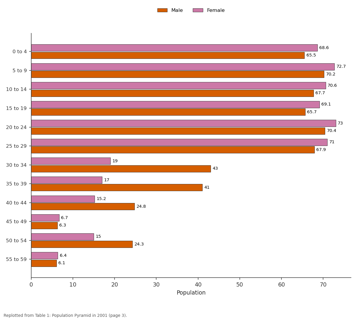
Male and Female: 0 to 4 vs 5 to 9 vs 10 to 14 vs 15 to 19 vs 20 to 24
Replotted from Table 1 (page 3) of the original paper. Every bar is the paper's own table value.
View source evidence ↗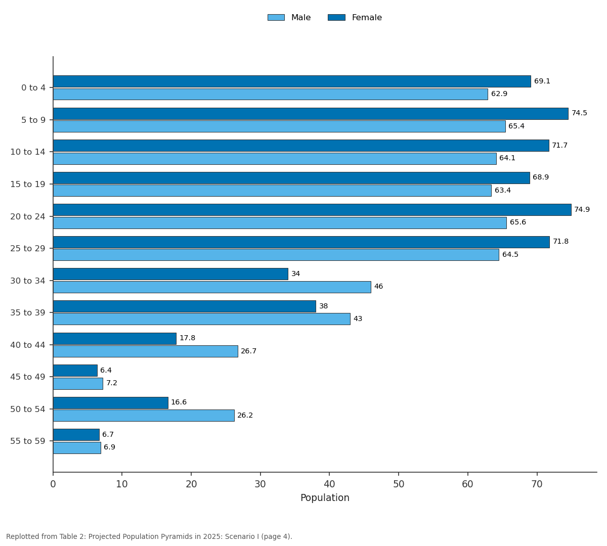
Male and Female: 0 to 4 vs 5 to 9 vs 10 to 14 vs 15 to 19 vs 20 to 24
Replotted from Table 2 (page 4) of the original paper. Every bar is the paper's own table value.
View source evidence ↗Figures & tables
From the original paper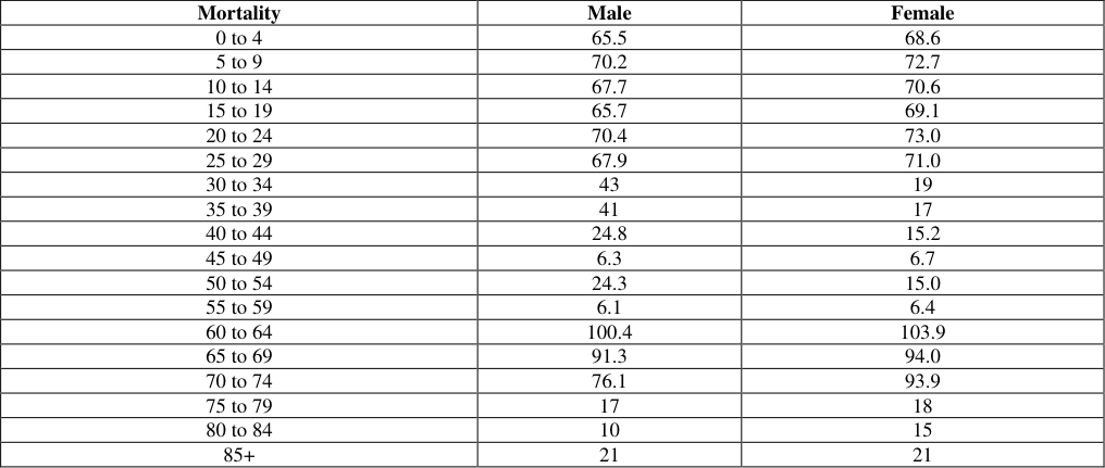 Table 1
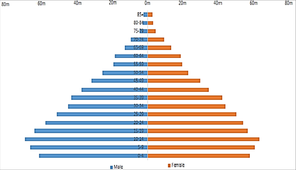 Figure 1
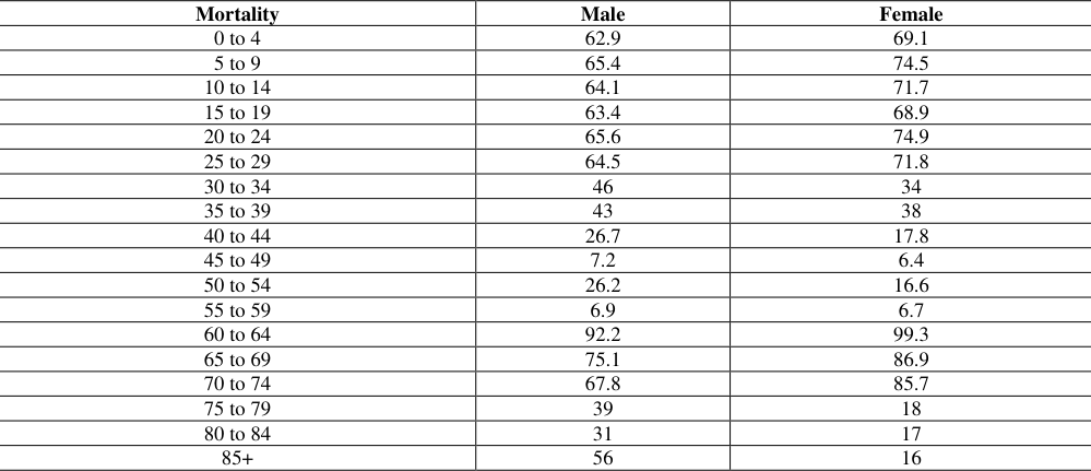 Table 2
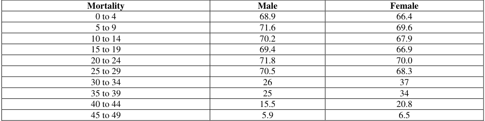 Table 3
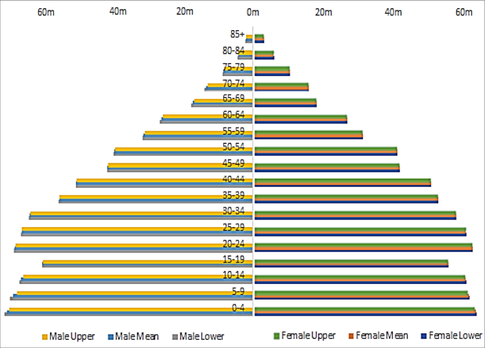 Figure 2
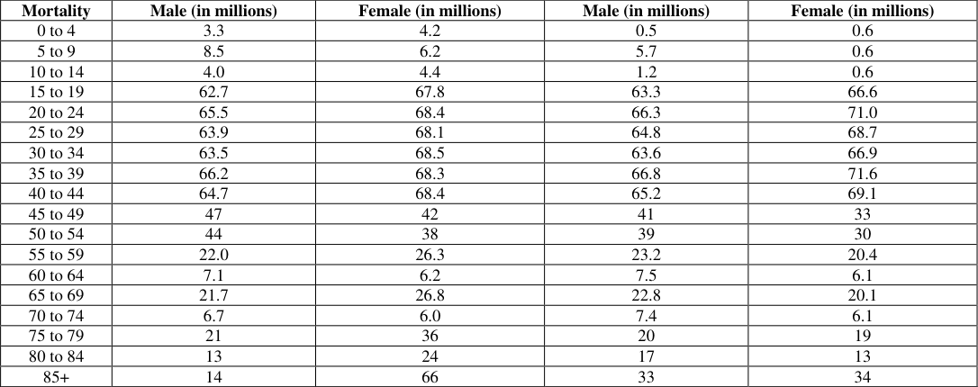 Table 4
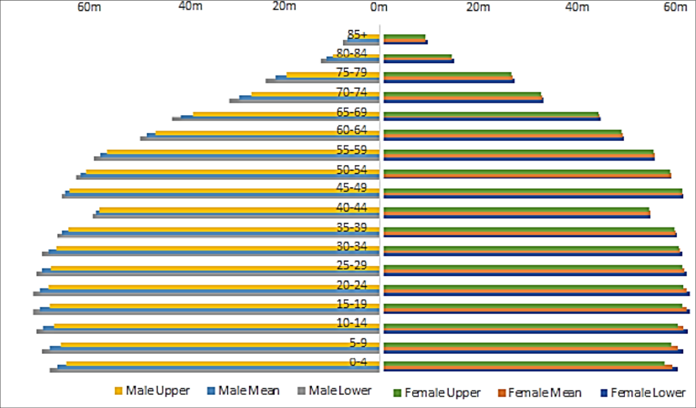 Figure 3
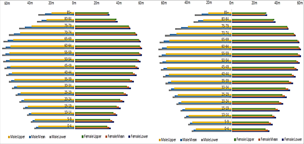 Figure 4
Introduction
The stochastic propagation of forecasting errors for mortality has its origins in the broader context of stochasticity of national population forecasting [1] . Some authors have made important contributions to mortality in national forecasts. Their results build on the works on general population forecasting published by many others [2] . Forecasts of the size and structure of the population are central to social and economic planning. Not least of the demographic challenges facing developed countries is the rapid ageing of the population. A full implementation of a stochastic forecast is a considerable task requiring a detailed analysis of the uncertainties of the jump-off population. Several different approaches to stochastic demographic forecasting have been developed in recent years [3] . The most widely used are those that involve some form of extrapolation, often using time series methods. Functional data methods fall into this category, but they have only recently been adopted in demographic forecasting. Functional data methods have the advantage of providing a flexible framework that can be used for all three demographic processes. In the present research work, using a new method for coherent mortality forecasting which involves forecasting interpretable product and ratio functions of rates using the functional data paradigm introduced in Hyndman and Ullah (2007) [4] . The product-ratio functional forecasting method can be applied to two or more sub-populations, incorporates convenient calculation of prediction intervals as well as point forecasts and is suitable for use within a larger stochastic population modeling framework such as Hyndman and Booth (2008) [5] .
Materials and Methods
The data required for analysis purpose, we mostly rely on secondary data which was obtained from census or SRS source. For analysis, two datasets in age-period format was required for males and females separately Central death rates (mx) = number of deaths/mid-year population (with a more complicated calculation for mx at age 0 reflecting the skewed distribution of deaths in the first year of life) Exposures to the risk of death (ie mid-year population). The central death rates for year ended 30 June; therefore 'mid-year' populations will at 31 December of the previous year. To deal with this efficiently in the analysis, we will try to simply shift the year in the population datasets, so that the year for the population is the same as the year for the mx value it relates to. For initial analysis we use actual data only by restricting our fitting period to the years 2001 to 2011.
In the functional data paradigm, we assume that there is an underlying smooth function f t,F (x) that we are observing with error. Thus,
where x i is the center of age group i (i 0 1, . . . p), E t,F,i is an independent and identically distributed standard normal random variable, and σ t,F (x i ) allows the amount of noise to vary with age x. Analogous notation is used for males. For smoothing, we use weighted penalized regression splines (Wood 1994) [6] constrained so that each curve is monotonically increasing above age x= 65 (Hyndman and Ullah 2007) [4] . The weights are to take care of the heterogeneity in death rates across ages. The observational variance σ t,F (x) is estimated by using a separate penalized regression spline of {yt(xi)log[f t,F (x i )]} 2 against x i , for each t.
We use functional time series models (Hyndman and Ullah 2007) 4 for p t (x) and r t (x):
where the functions {ϕ k (x)} and {ψ l (x)} are the principal components obtained from decomposing {pt(x)} and {rt(x)}, respectively, and β t,k and γ t,l are the corresponding principal component scores. The function μ p (x) is the mean of the set of curves {pt(x)}, and μ r (x) is the mean of {r t (x)}. The error terms, given by e t (x) and w t (x), have zero mean and are serially uncorrelated. The models are estimated using the weighted principal components algorithm of Hyndman and Shang [7] , which places more weight on recent data and so avoids the problem of the functions {ϕ k (x)} and {ψ l (x)} changing over time (Lee and Miller 2001) [8] . The coefficients, {βt,1,..., βt,K} and {gt,1,..., gt,L}, are forecast using time series models as detailed in the upcoming section on forecasts and prediction intervals. To ensure that the forecasts are coherent, we require the coefficients {gt,l} to be stationary processes. The forecast coefficients are then multiplied by the basis functions, resulting in forecasts of the curves pt(x) and rt(x) for future t. If pn+h|n(x) and rn+h|n(x) are h-step forecasts of the product and ratio functions, respectively, then forecasts of the sex-specific death rates are obtained using fn+h|n, M(x) 0 pn+h|n(x)rn+h|n(x) and fn+h|n, M(x) 0 pn+h|n(x)/rn+h|n(x). Forecasts are obtained by forecasting each coefficient βt, 1,..., βt,K and γt,1,..., γt,L independently. There is no need to consider vector models because the βt,k coefficients are all uncorrelated by construction (see Hyndman and Ullah 2007) [4] , as are the γt,l coefficients. They are also approximately uncorrelated with each other because of the use of products and ratios. The coefficients of the product model, {βt,1,..., βt,K}, are forecast using possibly non stationary autoregressive integrated moving average (ARIMA) models (Shumway and Stoffer 2006) [9] without restriction. When fitting ARIMA models, we use the automatic model selection algorithm given by Hyndman and Khandakar (2008) [10] to select the appropriate model orders. The coefficients of the ratio model, {gt,1,j, gt,2, j,..., gt,L,j}, j 0 1,2, . . . , J, are each forecast using any stationary autoregressive moving average (ARMA)(p,q) (Box et al. 2008) [11] or autoregressive fractionally integrated moving-average (ARFIMA) (p,d,q) process (Granger and Joyeux 1980; Hosking 1981) [12,13] . The stationarity requirement ensures that the forecasts are coherent. We have found ARFIMA models useful for forecasting the ratio function coefficients because they provide for longer-memory behavior than is possible with ARMA models. In implementing ARFIMA (p,d,q) models, we estimate the fractional differencing parameter d using the method of Haslett and Raftery (1989) [14] , we use the algorithm of Hyndman and Khandakar (2008) [14] to choose the orders p and q, and then we use maximum-likelihood estimation (Haslett and Raftery 1989) [10] and the forecast equations of Peiris and Perera (1988) [15] . In the stationary ARFIMA models, -0.5 < d < .05 for d 0 0; and the ARFIMA (p,d,q) model is equivalent to an ARMA(p,q) model. Let ∧ denote the h-step-ahead forecast of βn+h,k, and let ∧ denote the h step-ahead forecast of γn+h,l, j. Then the h-step-ahead forecast of log mn+h, j(x) is given by
Because all terms are uncorrelated, we can simply add the variances together so that where I n denotes all observed data up to time n plus the basis functions {ϕk(x)} and {ψl(x)}; un+h|n,k 0 var (βn+h,k|β1,k, …, βn,k) and vn+h|n,k 0 var (γn+h,k|γ1,k , …, γn,K) can be obtained from the time series models; σˆ μ j x 2 (x) (the variances of the smoothed means) can be obtained from the smoothing method used; se(x) is estimated by averaging e x ˆ t 2 (x) for each x; and sw,j(x) is estimated by averaging ˆt j , 2 w x(x) for each x. The observational variance σt j x, 2 (x) is very stable from year to year, and so it is estimated by taking the mean observational variance in the historical data. A prediction interval is then easily constructed under the assumption that the errors are normally distributed. Life expectancy forecasts are obtained from the forecast agespecific death rates using standard life table methods (Preston et al. 2001) [16] . To obtain prediction intervals for life expectancies, we simulate a large number of future death rates, as described in Hyndman and Booth (2008) [5] , and obtain the life expectancy for each. Then the prediction intervals are constructed from percentiles of these simulated life expectancies.
Results and Discussion
The application of the functional coherent model in projecting stochastic population forecasting through population pyramid.
A population pyramid is a diagram that provides a graphical illustration of the age distribution of a population, separately for the male and female, respectively in the left and the right side of the diagram. India's population pyramid in 2001 is depicted in below table 1 and Figure 1. As a first step towards building the projected population pyramid, the functional coherent model is extended onto mortality rates in India. Next, the forecasted birth rates are multiplied by the total population of the previous year to estimate the population added in that particular year. We have also built 95% confidence intervals around histograms of the pyramids based on lower and upper limits of the forecasted mortalities. In this manner, projected pyramids can be constructed for any of the years in the forecast horizon, for each of the two scenarios for future gender ratios at birth. For demonstration, we have chosen to show the projected pyramids for three of these years: 2025, 2050 and 2100. Below Table 2 and Figure 2 shows the predicted pyramids (along with 95% confidence intervals) for 2025, projected under Scenario I for gender ratio at birth. The anticipated population pyramid in 2100 is shown in Table 4 and Figure 4 below, under both scenarios of projected gender ratio at birth. While there is some difference in the projected pyramids between the two scenarios, as we can see from Above two figures, it is quite nominal. Such differences are naturally even less for the year 2025 and 2050.
| Mortality | Male (in millions) | Female (in millions) | Male (in millions) | Female (in millions) |
|---|---|---|---|---|
| 0 to 4 | 3.3 | 4.2 | 0.5 | 0.6 |
| 5 to 9 | 8.5 | 6.2 | 5.7 | 0.6 |
| 10 to 14 | 4.0 | 4.4 | 1.2 | 0.6 |
| 15 to 19 | 62.7 | 67.8 | 63.3 | 66.6 |
| 20 to 24 | 65.5 | 68.4 | 66.3 | 71.0 |
| 25 to 29 | 63.9 | 68.1 | 64.8 | 68.7 |
| 30 to 34 | 63.5 | 68.5 | 63.6 | 66.9 |
| 35 to 39 | 66.2 | 68.3 | 66.8 | 71.6 |
| 40 to 44 | 64.7 | 68.4 | 65.2 | 69.1 |
| 45 to 49 | 47 | 42 | 41 | 33 |
| 50 to 54 | 44 | 38 | 39 | 30 |
| 55 to 59 | 22.0 | 26.3 | 23.2 | 20.4 |
| 60 to 64 | 7.1 | 6.2 | 7.5 | 6.1 |
| 65 to 69 | 21.7 | 26.8 | 22.8 | 20.1 |
| 70 to 74 | 6.7 | 6.0 | 7.4 | 6.1 |
| 75 to 79 | 21 | 36 | 20 | 19 |
| 80 to 84 | 13 | 24 | 17 | 13 |
| 85+ | 14 | 66 | 33 | 34 |
Table text extracted from the original PDF; superscript letters are shown inline. The original table image is below.
View original table image
| Mortality | Male | Female |
|---|---|---|
| 0 to 4 | 62.9 | 69.1 |
| 5 to 9 | 65.4 | 74.5 |
| 10 to 14 | 64.1 | 71.7 |
| 15 to 19 | 63.4 | 68.9 |
| 20 to 24 | 65.6 | 74.9 |
| 25 to 29 | 64.5 | 71.8 |
| 30 to 34 | 46 | 34 |
| 35 to 39 | 43 | 38 |
| 40 to 44 | 26.7 | 17.8 |
| 45 to 49 | 7.2 | 6.4 |
| 50 to 54 | 26.2 | 16.6 |
| 55 to 59 | 6.9 | 6.7 |
| 60 to 64 | 92.2 | 99.3 |
| 65 to 69 | 75.1 | 86.9 |
| 70 to 74 | 67.8 | 85.7 |
| 75 to 79 | 39 | 18 |
| 80 to 84 | 31 | 17 |
| 85+ | 56 | 16 |
Table text extracted from the original PDF; superscript letters are shown inline. The original table image is below.
View original table image
| Mortality | Male | Female |
|---|---|---|
| 0 to 4 | 65.5 | 68.6 |
| 5 to 9 | 70.2 | 72.7 |
| 10 to 14 | 67.7 | 70.6 |
| 15 to 19 | 65.7 | 69.1 |
| 20 to 24 | 70.4 | 73.0 |
| 25 to 29 | 67.9 | 71.0 |
| 30 to 34 | 43 | 19 |
| 35 to 39 | 41 | 17 |
| 40 to 44 | 24.8 | 15.2 |
| 45 to 49 | 6.3 | 6.7 |
| 50 to 54 | 24.3 | 15.0 |
| 55 to 59 | 6.1 | 6.4 |
| 60 to 64 | 100.4 | 103.9 |
| 65 to 69 | 91.3 | 94.0 |
| 70 to 74 | 76.1 | 93.9 |
| 75 to 79 | 17 | 18 |
| 80 to 84 | 10 | 15 |
| 85+ | 21 | 21 |
Table text extracted from the original PDF; superscript letters are shown inline. The original table image is below.
View original table image
After analysing stochastic population forecasting by using coherent demographic model, the projected evolution of the population pyramids reveals several insightful information.
There is gradual narrowing of base reflecting reduction in birth rate. The gradual bulge towards the top is reflective of reduced mortality across ages. The four pyramids show how India is likely to progress towards being like other aging population by the end of the century.
For analysing stochastic population forecasting by using coherent demographic model, the results showed a life expectancy at birth in 2037 of 86.4 years for females and 82.9 years for males. The forecast sex gap decreases from 4.0 years in 2007 to 3.5 years in 2037. Similarly, for life expectancy at all other ages, the forecast sex gap decreases with slow convergence toward positive values. The forecast life expectancies at birth in 2037 imply average annual increments of 0.113 years for females and 0.138 years for males. These are less than the average annual increments over the fitting period, implying deceleration in the rate of increase. For females, deceleration is in fact observed over the fitting period and is continued in the forecast. Bengtsson (2019) [17] noted that deceleration has been a recent feature of several formerly leading countries of female life expectancy. For males, the linear trend since 2006 in observed life expectancy is not continued in the forecast. When linearity is continued in the forecast of the coefficient, it does not produce linearity in forecast life expectancy. The main reason for this is that the principal component model assumes a fixed age pattern of change, whereas life expectancy takes into account the fact that the age pattern of change varies over time (Booth et al. 2008) [18] . The pessimistic forecast is based on a functional model using a single principal component with linear coefficient, and hence a fixed age pattern of change. The optimistic forecast is a random walk with drift model of life expectancy. This latter model is heavily dependent on the fitting period and in particular on the first year of the fitting period. If we were to discount the first few years of the fitting period, when the trend is particularly steep, a more gradual increase in forecast life expectancy would result, but this would still be greater than the increase embodied in the single principal component model.
Coherent forecasting incorporates additional information into the forecast for a single population. The additional information acts as a frame of reference, limiting the extent to which a subpopulation forecast may continue a trend that differs from that of trends in related subpopulations.
It has been shown that the product-ratio functional method ensures non-divergence without compromising the overall (average) accuracy of the forecasts. In the two-sex case, the accuracy of the male mortality forecast was improved at the expense of accuracy in female mortality forecast; in other words, by adopting the coherent method, the accuracy of the forecasts for the two sexes was (partly) equalized. Similarly in the six-state example, forecast accuracy is more homogeneous in the coherent method, with an improvement in overall accuracy. This feature of the method is useful in practical applications such as population forecasting, where it is preferable to maintain a balanced margin of error and hence a more balanced forecast population structure than might occur in the independent case. Similarly in financial planning, it may be preferable to accept moderate error in all subpopulations rather than risk a large error in one subpopulation. Coherent forecasting incorporates additional information into the forecast for a single subpopulation. The additional information acts as a frame of referencelimiting the extent to which a subpopulation forecast may continue a trend that differs from that of trends in related subpopulations.
A similar approach has previously been adopted in forecasting fertility and for mortality [19] . Evidence suggests that the product-ratio functional method may produce more accurate forecasts than other methods. The evaluations show that the functional data model of this study produces more accurate forecasts of death rates than the Lee Carter method and its variants in 13 out of 20 populations. In this research we have used an improved functional data model which incorporates weights and has been shown to produce more accurate forecasts than any other method based on a principal components decomposition including the Lee-Carter variant used by Li and Lee 2005 [20] .
The development of improved forecasting methods for mortality represents a step toward more reliable and more easily automated demographic forecasting and the acceptance of these stochastic methods by national statistical offices responsible for producing official population projections. Although more complex than traditional methods was there, these methods are easily accessible through user-friendly code now available on the Comprehensive R Archive Network (CRAN). Application of the methods is considerably simplified by this free software. The coherent LC method worked well for the India population. It gave a reasonable mortality forecast in the context of a plausible age pattern of mortality decline and sex differentials. Even though the coherent LC method did not make much of a difference in terms of sex-combined life expectancies at birth, comparing the separate LC method, it still improved the mortality forecasting by age and sex and was comparable to other populations of East Asia with precedent and similar experiences.
Conclusion
In conclusion, the development of improved mortality forecasting methods, and by extension, fertility and migration forecasting methods, represents a step toward more reliable and automated demographic forecasting.
Figures and tables from the paper
| Mortality | Male | Female |
|---|---|---|
| 0 to 4 | 68.9 | 66.4 |
| 5 to 9 | 71.6 | 69.6 |
| 10 to 14 | 70.2 | 67.9 |
| 15 to 19 | 69.4 | 66.9 |
| 20 to 24 | 71.8 | 70.0 |
| 25 to 29 | 70.5 | 68.3 |
| 30 to 34 | 26 | 37 |
| 35 to 39 | 25 | 34 |
| 40 to 44 | 15.5 | 20.8 |
| 45 to 49 | 5.9 | 6.5 |
Table text extracted from the original PDF; superscript letters are shown inline. The original table image is below.
View original table image
References
20 in the original paper- Martínez-Ruiz F, Mateu J, Montes F, Porcu E. Mortality risk assessment through stationary space-time covariance functions. Stochastic Environmental Research and Risk Assessment. 2010 May 1;24(4):519-26
- Giacometti R, Bertocchi M, Rachev ST, Fabozzi FJ. A comparison of the Lee-Carter model and AR-ARCH model for forecasting mortality rates. Insurance: Mathematics and Economics. 2012 Jan 1;50(1):85-93.
- Booth H. Demographic forecasting: 1980 to 2005 in review. International journal of forecasting. 2006 Jan 1;22(3):547-81.
- Hyndman RJ, Ullah MS. Robust forecasting of mortality and fertility rates: A functional data approach. Computational Statistics & Data Analysis. 2007 Jun 15;51(10):4942-56.
- Hyndman RJ, Booth H. Stochastic population forecasts using functional data models for mortality, fertility and migration. International Journal of Forecasting. 2008 Jul 1;24(3):323-42.
- Wood SN. Monotonic smoothing splines fitted by cross validation. SIAM Journal on Scientific Computing. 1994 Sep;15(5):1126-33.
- Hyndman RJ, Shang HL. Rainbow plots, bagplots, and boxplots for functional data. Journal of Computational and Graphical Statistics. 2010 Jan 1;19(1):29-45.
- Lee R, Miller T. Evaluating the performance of the LeeCarter method for forecasting mortality. Demography. 2001 Nov;38(4):537-49.
- Shumway RH, Stoffer DS. Spectral analysis and filtering. Time series analysis and its applications: With r examples, 2006, 174-270.
- Hyndman RJ, Khandakar Y. Automatic time series forecasting: the forecast package for R. Journal of statistical software. 2008 Jul 29;27:1-22.
- Box GE, Jenkins GM, Reinsel GC, Ljung GM. Time series analysis: forecasting and control. John Wiley & Sons; 2015 May 29.
- Granger CW, Joyeux R. An introduction to long-memory time series models and fractional differencing. Journal of time series analysis. 1980 Jan;1(1):15-29.
- Hosking JR. Fractional differencing modeling in hydrology 1. JAWRA Journal of the American Water Resources Association. 1985 Aug;21(4):677-82.
- Haslett J, Raftery AE. Space-time modelling with long-memory dependence: Assessing Ireland's wind power resource. Journal of the Royal Statistical Society: Series C (Applied Statistics). 1989 Mar;38(1):1-21.
- Peiris MS, Perera BJ. On prediction with fractionally differenced ARIMA models. Journal of Time Series Analysis. 1988 May;9(3):215-20.
- Preston SH, Heuveline P, Guillot M. [Book Review] demography, measuring and modeling population processes. Population and Development Review. 2001;27(2):365-7.
- Bengtsson T, Keilman N. Old and new perspectives on mortality forecasting. Springer Nature, 2019.
- Booth H, Tickle L. Mortality modelling and forecasting: A review of methods. Annals of actuarial science. 2008 Sep;3(1-2):3-43.
- Kim SY. Mortality forecasting for the republic of Korea: the Coherent Lee-Carter method. Korea Journal of population studies. 2011;34(3):157-77.
- Li N, Lee R. Coherent mortality forecasts for a group of populations: an extension of the Lee-Carter method. Demography. 2005;42(3):575-594.