
Research article · 2022 · Full text
International Journal of Statistics and Applied MathematicsConstruction and selection of double inspection quick switching system
Volume 7(2) · Pages 105–107 · DOI: 10.22271/maths.2022.v7.i2b.802 ↗
Research areasAdvanced Statistical Process MonitoringIndustrial Vision Systems and Defect Detection
Abstract
Author-writtenAcceptance sampling plan have been widely used in industry to determine whether the manufactured item satisfy the pre-specified quality levels or not. At this point, an industry must have to take a decision for accepting or rejecting the lots in accordance with randomly chosen units. In this article describes the quick switching system with the reference of double inspection single sampling plan. Tables are constructed for easy selection of sample size.
Summary
Source-checkedPlain-language reading of the full paper, prepared with AI and checked against the text. Each point links to the authors' own words.
Why it matters
- Acceptance sampling plans are common industrial tools used to decide if manufactured items meet specific quality standards. View evidence ↗
- Quick Switching Systems (QSS) use tightened inspection for poor quality and normal inspection with smaller samples for good quality. View evidence ↗
- Double inspection plans are particularly useful for high-volume or expensive production where higher quality assurance is required. View evidence ↗
The question
- The study aims to develop a Double Inspection Quick Switching System [DIQSS (0,1)] based on a Poisson model, using acceptance numbers of 0 for tightened and 1 for normal levels. View evidence ↗
What they did
- The double inspection process is designed so that the first inspection is independent of the second, continuing until a final decision to accept or reject the lot is made. View evidence ↗
- The first inspection phase involves checking for defectives at a normal level; if they exceed the limit (cN), the system shifts to a tightened level (cT) before deciding whether to proceed to the second inspection or reject the lot. View evidence ↗
- The second inspection phase follows a similar logic, where the lot is finally accepted only if the number of defectives at the tightened level (d22) is less than or equal to cT. View evidence ↗
- The authors used specific plan parameters of sample size n=41, normal acceptance number cN=2, and tightened acceptance number cT=1 to generate the system's characteristic curves. View evidence ↗
What they found
- At a fraction defective (p) of 0.001, the DIQSS probability of acceptance is 0.999978 with an Average Outgoing Quality (AOQ) of 0.001000. View evidence ↗
- When the fraction defective (p) increases to 0.05, the probability of acceptance drops to 0.289699 and the AOQ is 0.014485. View evidence ↗
- At a high fraction defective (p) of 0.1, the probability of acceptance is very low at 0.009643, with an AOQ of 0.000964. View evidence ↗
What it means
- The authors conclude that the Double Inspection Quick Switching Sampling system is an effective tool for consumers to ensure they receive high-quality products. View evidence ↗
Visual summary
3 visualsIllustrations explain the paper; charts are replotted from the paper's own table values.
DIQSS Decision Flowchart
AI-generated conceptual illustration (industrial quality control inspection line with mechanical parts). It explains the idea and does not show study data.
View source evidence ↗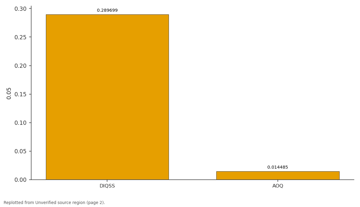
0.05: DIQSS vs AOQ
Replotted from a table (page 2) of the original paper. Every bar is the paper's own table value.
View source evidence ↗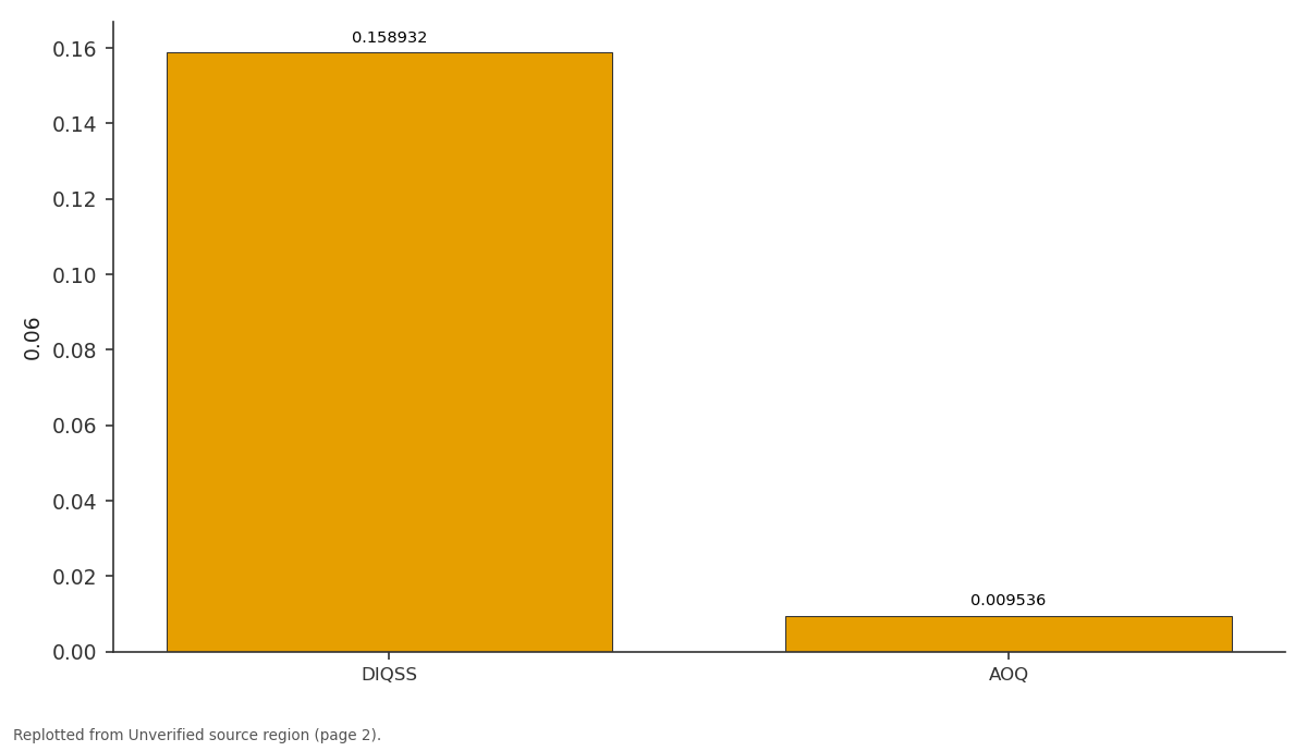
0.06: DIQSS vs AOQ
Replotted from a table (page 2) of the original paper. Every bar is the paper's own table value.
View source evidence ↗Figures & tables
From the original paper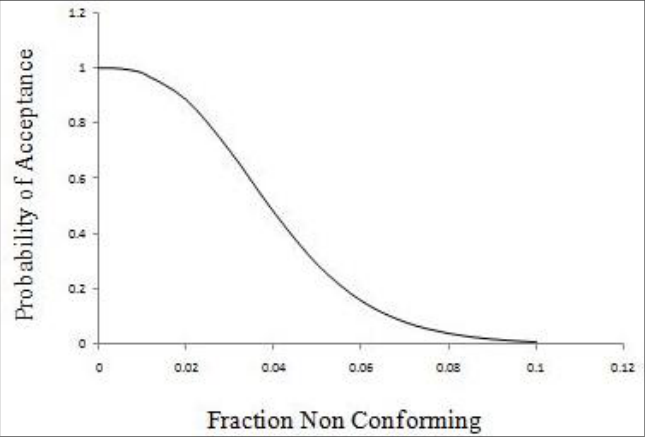 Figure 1
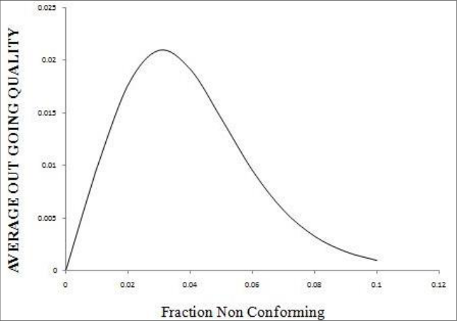 Figure 2
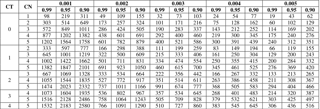 Table 1
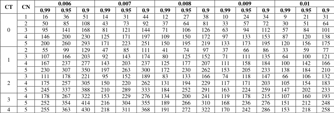 Table 1
Introduction
Dodge (1967) [1] has introduced new type of sampling system, which consists of pairs of normal and tightened plans, other sampling systems the inspection involving only normal and tightened inspection is usually referred as two-plan system. The system considers tightened inspection plans for the poor quality levels and normal plans involving smaller sample size for the good quality levels. Due to instantaneous switching between normal and tightened plan this system is referred as “Quick Switching System”. After many authors extended and applied Quick Switching Sampling System in various branches of statistical quality control.
Romboski introduced QSS-1 (n;cN,cT) which is a QSS-1 with single sampling plan as a reference plan [(n,cN), (n,cT) respectively the normal and tightened single sampling plans with cT < cN], Soundarrajan and Devaraj Arumai Nayagam (1990) [10] have developed Construction and Selection of Modified Quick Switching System. Govindaraju and Subramani (1990) [2] have developed Selection of Single-sampling Quick Switching System for given Acceptable and Limiting Quality Levels. Soundarrajan and Devaraj Arumai Nayagam (1992) [11] have developed Quick switching system for costly and destructive testing. Senthilkumar et al. (2012) [4] have developed Construction of quick switching variable sampling system indexed by cross over point.
Senthilkumar et al. (2018) [5] developed Construction of modified quick switching variable sampling system indexed by crossover Point. Vennila and Devaraj Arumainayagam (2018) [12] have developed Quick Switching System with different reference plans. Senthilkumar and Sabarish (2020) [6] have developed the Construction and Selection of Double Inspection Single Sampling Plan [DISSP (0,1)]. Senthilkumar and Sabarish (2021) [7, 8] have developed Selection and Development of Double Inspection Single Sampling Plan.
Senthilkumar and Sabarish (2021) [7, 8] have developed Economic Design of Double Inspection Single Sampling Plan. The work presented in this paper is Double Inspection Quick Switching System with acceptance number 0 for tightened level and 1 for normal level [DIQSS (0,1)] with reference to single sampling plan based on the poisson model. In double inspection, the first inspection does not depend on second inspection, the inspection process has to be continued until the lot is either accepted or rejected. Operating Procedure Select the random sample ‘n’ from the population ‘N’ 1.
Select a random sample of size ‘n’ units from the lot and test each unit for conformance to the specified attribute requirements. Maths 2022; 7(2): 105-107 D Senthilkumar Department of Statistics, PSG College of Arts & Science, Coimbatore, Tamil Nadu, India P Sabarish Department of Statistics, PSG College of Arts & Science, Coimbatore, Tamil Nadu, India D Senthilkumar Department of Statistics, PSG College of Arts & Science, Coimbatore, Tamil Nadu, India http://www.mathsjournal.com 2. In first inspection find the number of defective d11 at normal level if d11 ≤ cN move to second inspection otherwise shift to tighten level. 3. Count the number of defectives ‘d12’ at the tighten level if d12≤ cT move to second inspection otherwise reject the lot. 4.
In second inspection find the number of defective d21 at day. In DIQSS two inspectors checking two different quality Characteristics of the Smart ring with Normal and Tighten level, c11= Checking quality of the display and c12 = Checking the performance of the Sensor, both the quality characteristics are independent (Normal). c21= Checking quality of the display and c22 = Checking the performance of the Sensor, both the quality characteristics are independent (tighten). normal level if d21 ≤ cN move to second inspection otherwise shift to tighten level. 5. Count the number of defectives ‘d22’ at the tighten level if d22≤ cT accept the lot otherwise reject the lot. Operating Characteristics Function Pa (p) = [Pa1(p) = PT PT+ (1−PN)] [Pa2(p) = PT PT+ (1−PN)] p DIQSS AOQ 0.001 0.999978 0.001000 0.003 0.999430 0.002998 0.005 0.997494 0.004987 0.007 0.993444 0.006954 0.009 0.986684 0.008880 0.01 0.982133 0.009821 0.02 0.885310 0.017706 0.03 0.700305 0.021009 0.04 0.480036 0.019201 0.05 0.289699 0.014485 0.06 0.158932 0.009536 0.07 0.081952 0.005737 0.08 0.040771 0.003262 0.09 0.019912 0.001792 0.1 0.009643 0.000964 Average outgoing Quality AOQ = p( Pa (p)) Illustration In the digital world usage of the smart products (smart phone, smart watch, smart bag, smart glass...etc.) increase day by Fig 1: Operating characteristics curve Fig 2: Average outgoing quality curve http://www.mathsjournal.com Figure 1 reflects the operating characteristics curve of Double Inspection Quick Switching System and Figure 2 reflects the Average Outgoing Quality curve of Double Inspection Quick Switching System.
These curves formed by the plan parameters n=41, cN=2 and cT=1 and points of the curves are shown in the Table 1. Table 1: locates the values of sample size n, this sample size ‘n’ is indexed by the parameters p, cT, cN and Pa (p). CT CN 0.001 0.002 0.003 0.004 0.005 0.99 0.95 0.90 0.99 0.95 0.90 0.99 0.95 0.90 0.99 0.95 0.90 0.99 0.95 0.90 0 1 98 219 311 49 109 155 32 73 103 24 54 77 19 43 62 2 303 514 649 173 257 324 101 171 216 75 128 162 60 102 129 3 572 849 1011 286 424 505 190 283 337 143 212 252 114 169 202 4 877 1202 1382 438 601 691 292 400 460 219 300 345 175 240 276 5 1202 1564 1758 601 782 879 400 521 586 300 391 439 240 312 351 1 2 333 597 777 166 298 388 111 199 259 83 149 194 66 119 155 3 645 1001 1219 322 500 609 215 333 406 161 250 304 129 200 243 4 1002 1422 1662 501 711 831 334 474 554 250 355 415 200 284 332 5 1382 1847 2101 691 923 1050 460 615 700 345 461 525 276 369 420 2 3 667 1069 1328 333 534 664 222 356 442 166 267 332 133 213 265 4 1055 1544 1835 527 772 917 351 514 611 263 386 458 211 308 367 5 1474 2023 2332 737 1011 1166 991 674 777 368 505 583 294 404 466 3 4 1073 1604 1935 536 802 967 357 534 645 268 401 483 214 320 387 5 1516 2128 2486 758 1064 1243 505 709 828 379 532 621 303 425 497 4 5 1532 2183 2580 766 1091 1290 510 727 860 383 545 645 306 436 516 Table 1: Continued….. CT CN 0.006 0.007 0.008 0.009 0.01 0.99 0.95 0.9 0.99 0.95 0.9 0.99 0.95 0.9 0.99 0.95 0.9 0.99 0.95 0.9 0 1 16 36 51 14 31 44 12 27 38 10 24 34 9 21 31 2 50 85 108 43 73 92 37 64 81 33 57 72 30 51 64 3 95 141 168 81 121 144 71 106 126 63 94 112 57 84 101 4 146 200 230 125 171 197 109 150 172 97 133 153 87 120 138 5 200 260 293 171 223 251 150 195 219 133 173 195 120 156 175 1 2 55 99 129 47 85 111 41 74 97 37 66 86 33 59 77 3 107 166 203 92 143 174 80 125 152 71 111 135 64 100 121 4 167 237 277 143 203 237 125 177 207 111 158 184 100 142 166 5 230 307 350 197 263 300 172 230 262 153 205 233 138 184 210 2 3 111 178 221 95 152 189 83 133 166 74 118 147 66 106 132 4 175 257 305 150 220 262 131 194 229 117 171 203 105 154 183 5 245 337 388 210 289 333 184 252 291 163 224 259 147 202 233 5.
| CT | CN | 0.006 | — | — | 0.007 | — | — | 0.008 | — | — | 0.009 | — | — | 0.01 | — | — |
|---|---|---|---|---|---|---|---|---|---|---|---|---|---|---|---|---|
| 0.99 | 0.95 | 0.9 | 0.99 | 0.95 | 0.9 | 0.99 | 0.95 | 0.9 | 0.99 | 0.95 | 0.9 | 0.99 | 0.95 | 0.9 | ||
| 0 | 1 | 16 | 36 | 51 | 14 | 31 | 44 | 12 | 27 | 38 | 10 | 24 | 34 | 9 | 21 | 31 |
| 2 | 50 | 85 | 108 | 43 | 73 | 92 | 37 | 64 | 81 | 33 | 57 | 72 | 30 | 51 | 64 | |
| 3 | 95 | 141 | 168 | 81 | 121 | 144 | 71 | 106 | 126 | 63 | 94 | 112 | 57 | 84 | 101 | |
| 4 | 146 | 200 | 230 | 125 | 171 | 197 | 109 | 150 | 172 | 97 | 133 | 153 | 87 | 120 | 138 | |
| 5 | 200 | 260 | 293 | 171 | 223 | 251 | 150 | 195 | 219 | 133 | 173 | 195 | 120 | 156 | 175 | |
| 1 | 2 | 55 | 99 | 129 | 47 | 85 | 111 | 41 | 74 | 97 | 37 | 66 | 86 | 33 | 59 | 77 |
| 3 | 107 | 166 | 203 | 92 | 143 | 174 | 80 | 125 | 152 | 71 | 111 | 135 | 64 | 100 | 121 | |
| 4 | 167 | 237 | 277 | 143 | 203 | 237 | 125 | 177 | 207 | 111 | 158 | 184 | 100 | 142 | 166 | |
| 5 | 230 | 307 | 350 | 197 | 263 | 300 | 172 | 230 | 262 | 153 | 205 | 233 | 138 | 184 | 210 | |
| 2 | 3 | 111 | 178 | 221 | 95 | 152 | 189 | 83 | 133 | 166 | 74 | 118 | 147 | 66 | 106 | 132 |
| 4 | 175 | 257 | 305 | 150 | 220 | 262 | 131 | 194 | 229 | 117 | 171 | 203 | 105 | 154 | 183 | |
| 5 | 245 | 337 | 388 | 210 | 289 | 333 | 184 | 252 | 291 | 163 | 224 | 259 | 147 | 202 | 233 | |
| 3 | 4 | 178 | 267 | 322 | 153 | 229 | 276 | 134 | 200 | 241 | 119 | 178 | 215 | 107 | 160 | 193 |
| 5 | 252 | 354 | 414 | 216 | 304 | 355 | 189 | 266 | 310 | 168 | 236 | 276 | 151 | 212 | 248 | |
| 4 | 5 | 255 | 363 | 430 | 218 | 311 | 368 | 191 | 272 | 322 | 170 | 242 | 286 | 153 | 218 | 258 |
Table text extracted from the original PDF; superscript letters are shown inline. The original table image is below.
View original table image
| CT | CN | 0.001 | — | — | 0.002 | — | — | 0.003 | — | — | 0.004 | — | — | 0.005 | — | — |
|---|---|---|---|---|---|---|---|---|---|---|---|---|---|---|---|---|
| 0.99 | 0.95 | 0.90 | 0.99 | 0.95 | 0.90 | 0.99 | 0.95 | 0.90 | 0.99 | 0.95 | 0.90 | 0.99 | 0.95 | 0.90 | ||
| 0 | 1 | 98 | 219 | 311 | 49 | 109 | 155 | 32 | 73 | 103 | 24 | 54 | 77 | 19 | 43 | 62 |
| 2 | 303 | 514 | 649 | 173 | 257 | 324 | 101 | 171 | 216 | 75 | 128 | 162 | 60 | 102 | 129 | |
| 3 | 572 | 849 | 1011 | 286 | 424 | 505 | 190 | 283 | 337 | 143 | 212 | 252 | 114 | 169 | 202 | |
| 4 | 877 | 1202 | 1382 | 438 | 601 | 691 | 292 | 400 | 460 | 219 | 300 | 345 | 175 | 240 | 276 | |
| 5 | 1202 | 1564 | 1758 | 601 | 782 | 879 | 400 | 521 | 586 | 300 | 391 | 439 | 240 | 312 | 351 | |
| 1 | 2 | 333 | 597 | 777 | 166 | 298 | 388 | 111 | 199 | 259 | 83 | 149 | 194 | 66 | 119 | 155 |
| 3 | 645 | 1001 | 1219 | 322 | 500 | 609 | 215 | 333 | 406 | 161 | 250 | 304 | 129 | 200 | 243 | |
| 4 | 1002 | 1422 | 1662 | 501 | 711 | 831 | 334 | 474 | 554 | 250 | 355 | 415 | 200 | 284 | 332 | |
| 5 | 1382 | 1847 | 2101 | 691 | 923 | 1050 | 460 | 615 | 700 | 345 | 461 | 525 | 276 | 369 | 420 | |
| 2 | 3 | 667 | 1069 | 1328 | 333 | 534 | 664 | 222 | 356 | 442 | 166 | 267 | 332 | 133 | 213 | 265 |
| 4 | 1055 | 1544 | 1835 | 527 | 772 | 917 | 351 | 514 | 611 | 263 | 386 | 458 | 211 | 308 | 367 | |
| 5 | 1474 | 2023 | 2332 | 737 | 1011 | 1166 | 991 | 674 | 777 | 368 | 505 | 583 | 294 | 404 | 466 | |
| 3 | 4 | 1073 | 1604 | 1935 | 536 | 802 | 967 | 357 | 534 | 645 | 268 | 401 | 483 | 214 | 320 | 387 |
| 5 | 1516 | 2128 | 2486 | 758 | 1064 | 1243 | 505 | 709 | 828 | 379 | 532 | 621 | 303 | 425 | 497 | |
| 4 | 5 | 1532 | 2183 | 2580 | 766 | 1091 | 1290 | 510 | 727 | 860 | 383 | 545 | 645 | 306 | 436 | 516 |
Table text extracted from the original PDF; superscript letters are shown inline. The original table image is below.
View original table image
Senthilkumar et al. Construction of Modified Quick Switching Variable Sampling System Indexed by Crossover Point. International Journal of Latest Engineering and Management Research. 2018;3(2):10- 18. 6. Senthilkumar, Sabarish.
Construction and Selection of Double Inspection Single Sampling Plan by Attributes [DISSP (0,1)]. International Journal of Disaster Recovery and Business Continuity. 2020;11(1):3295-3304. 7. Senthilkumar, Sabarish. Selection and Development of Double Inspection Single Sampling Plan.
Bulletin Monumental. 2021;22(5):7-12. 8. Senthilkumar, Sabarish. Economic Design of Double 3 4 178 267 322 153 229 276 134 200 241 119 178 215 107 160 193 5 252 354 414 216 304 355 189 266 310 168 236 276 151 212 248 4 5 255 363 430 218 311 368 191 272 322 170 242 286 153 218 258
Conclusion
The entries in Table 2 are the values of n. They are indexed by the parameters of cT and cN by Pa (p). In this paper, Double Inspection Quick Switching Sampling system that can help the consumer to get good quality products. Every sampling plan we are check single inspection for single quality characteristics of the product.
In costliest and high volume production we need extra caution about the product because we need more quality. In that situation we use Double Inspection Plan which is applicable for costliest and mass Production.
References
8 in the original paper- Dodge. A New Dual System of Acceptance Sampling Inspection Single Sampling Plan. GIS Science Journal. 2021;8:568-583.
- Senthilkumar, Sabarish. Design Of Double Inspection Technical report, No16 Statistics centre Rutgers: The State University, New Brunswick, New Jersey; c1967.
- Govindaraju, Subramani. Selection of Single-sampling Quick Switching System [DIQSS (0,1)]. International Journal of Mechanical Engineering. 2022;7(1):421-424.
- Soundarrajan, Devaraj Arumai Nayagam. Construction Quick Switching System for given Acceptable and Limiting Quality Levels International Journal of Quality and Reliability Management. 1990;8(2):45-51.
- Romboski. An Investigation of Quick Switching Acceptance Sampling Systems Ph.D. Dissertation. Rutgers: The State University, New Brunswick, New Jersey; c1969.
- Senthilkumar et al. Construction of Quick Switching and Selection of Modified Quick Switching System Journal of Applied Statistics. 1990;17(1):83-114.
- Soundarrajan, Devaraj Arumai Nayagam. Quick Switching System for Costly and Destructive Testing Sanakya: Indian Journal of Statistics. 1992;54(1):1-12.
- Vennila, Devaraj Arumainayagam. Quick Switching Variable Sampling System Indexed by Cross over Point. Technology. 2012;4(2):420-430. System with Different Reference Plans American Journal of Applied Mathematics and Statistics. 2018;6(4):141- 148.
Cited by 1
From OpenAlex, OpenCitations and reference lists read by Scinovex
- Constructing Optimal Quick Switching System with Hurdle Poisson Distribution ↗
Venugopal Haridoss, V Sasikala · Indian Journal of Science and Technology · 2024
Objectives: Optimizing the sum of risks involved in the selection of acceptance sampling plans playing a vital role. This paper uses the Hurdle Poisson distribution to design an optimal quick switching system attribute plan for a given acceptable quality level (AQL) and limiting quality level (LQL) involving a minimum sum of risks. Methods: The sum of producer's and consumer's risks…
❝ 0PDF