
Research article · 2022 · Full text
International Journal of Statistics and Applied MathematicsA study on analysis of reliability distributions
Volume 7(1) · Pages 118–121 · DOI: 10.22271/maths.2022.v7.i1b.781 ↗
Research areasReliability and Maintenance Optimization
Abstract
Author-writtenWhen we buy a mobile, laptop, scooter, car, or even a small item like bulb or battery, we can expect function satisfactory for a specific period of time. For this purpose one life testing experiments are wanted. These experiments are designed to find average life of an item or to ensure the questions like is the probability. The item will fail in time interval (t0, t0+t) such thing we will estimate reliability of the item through some continuous probability distributions.
Summary
Source-checkedPlain-language reading of the full paper, prepared with AI and checked against the text. Each point links to the authors' own words.
Why it matters
- Consumers expect products like electronics and vehicles to function satisfactorily for a specific duration of time. View evidence ↗
- Life testing experiments use continuous probability distributions to estimate an item's reliability and the probability of failure within a specific time interval. View evidence ↗
- Reliability distribution analysis describes the time to failure (TTF) using patterns such as Weibull, Normal, Lognormal, and Exponential distributions. View evidence ↗
The question
- The study aims to estimate the reliability of an item at a specific point in time. View evidence ↗
What they did
- The researchers calculated reliability using three specific reliability functions: Exponential, Weibull, and Lognormal distributions. View evidence ↗
- The analysis utilized a dataset with a total sum of 1184, tracking the number of failures and survivals over time in hours. View evidence ↗
- Descriptive statistics were calculated for the product, including a mean of 47.36, a median of 39.00, and a range from 20.00 to 130.00 hours. View evidence ↗
What they found
- At 1 hour, the reliability R(t) was 1.00, with 130 failures and 1184 survivals. View evidence ↗
- At 10 hours, the reliability R(t) dropped to 0.50, with 34 failures and 591 survivals. View evidence ↗
- By 25 hours, the reliability R(t) reached its minimum of 0.02, with 20 failures and 20 survivals. View evidence ↗
- Using the Lognormal distribution function at 1 hour, the reliability was calculated as 0.6784. View evidence ↗
- Using the Lognormal distribution function at 2 hours, the reliability was calculated as 0.532. View evidence ↗
What it means
- The authors conclude that the objective was achieved by outlining the reliability status of the studied extruder through functions and graphical representations. View evidence ↗
- The authors observed that reliability calculations start at 1 and end at 0, with a total failure density of one. View evidence ↗
Visual summary
2 visualsIllustrations explain the paper; charts are replotted from the paper's own table values.
Reliability Decay Concept
AI-generated conceptual illustration (industrial mechanical gear assembly). It explains the idea and does not show study data.
View source evidence ↗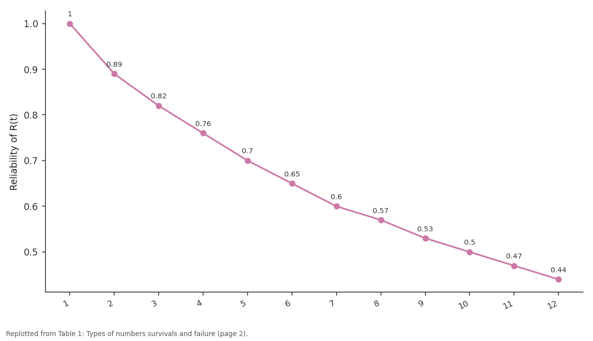
Reliability of R(t): 1 vs 2 vs 3 vs 4 vs 5
Replotted from Table 1 (page 2) of the original paper. Every bar is the paper's own table value.
View source evidence ↗Figures & tables
From the original paper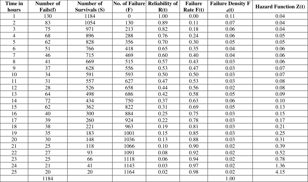 Table 1
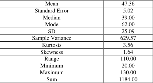 Table 2
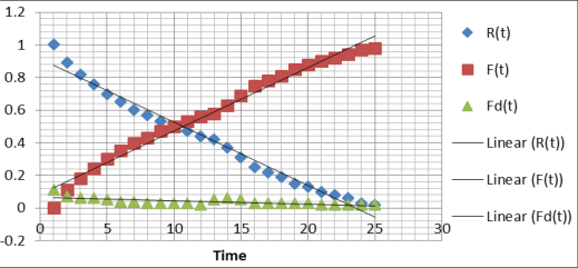 Figure 1
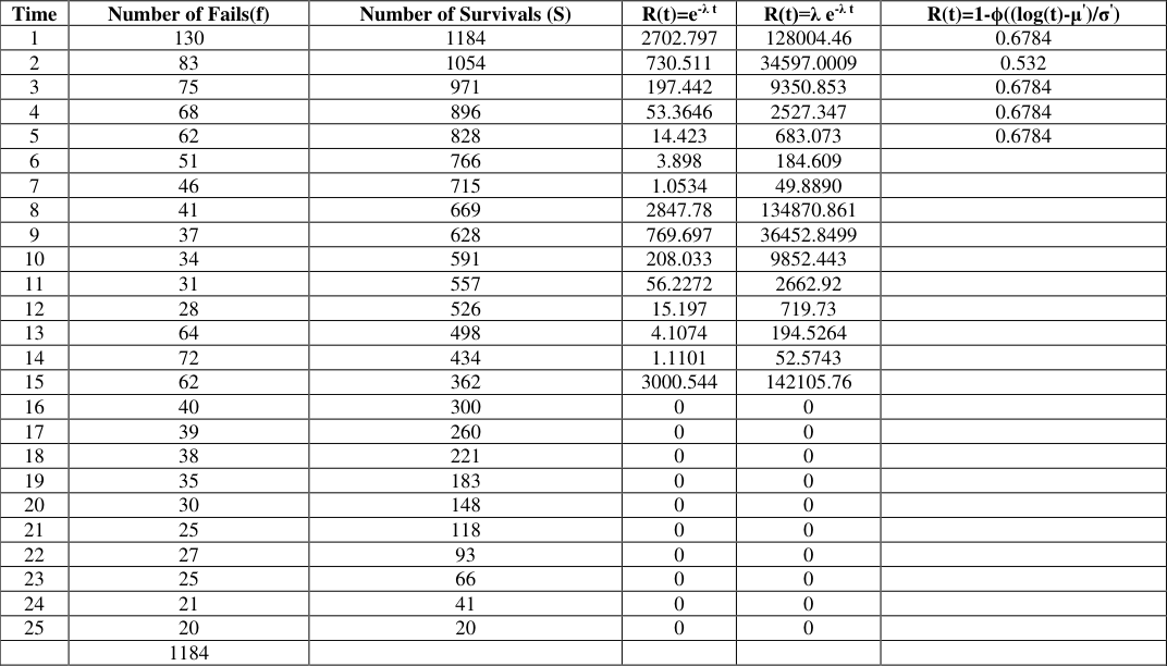 Table 3
Introduction
The reliability distributions are used to model random events for which the outcome is uncertain such as one time of failure for a component Artin E 1964 [1]. Before placing a demand on that component, the aim it will fail is unknown. The distribution of the probability of failure at different times is modelled by reliability distributions Dekking FM et al 2007 [2]. The reliability Distributions Analysis allows us to describe one time to failure (TTF) as a statistical distribution which is usually characterised by a specific pattern.
Four different “A” types are supported: Weibull, Normal, Long Normal, and Exponential Hastings NAJ et al. 2000 [3]. 2. Measures of reliability The most commonly used methods to measure the reliability are. a. Failure rate b. Probability of survival c.
Mean Time Between Failure d. Mean Time To Failure. 3. Failure rate The failure rate is defined as where in (iii) the ratio of number of failures during a particular unit interval to average population in that interval Meeker WQ et al. 1998 [4]. It is given by z(i) = ( 1) ( ) 2 s i si ni The failure rate is commonly expressed in terms of failures per hour or 100 hours (or) 1000hrs (or) percentage failures per 1000 hrs Meeker WQ et al. 1998 [5].
Sometimes the failure rate is represented by a Greek letter ‘ ’ and it is calculated as a simple ratio of total no. of failures during a specified test interval to total test hours. And it is given by f TotalNo.of failures t totaltesthours 1. Probability of survival: It indicates the probability or expected no. of items that will operate for a required period of time. and Maths 2022; 7(1): 118-121 G Vijaya Lakshmi Research Scholar, Department of Statistics, S.K. University, Anantapur, Andhra Pradesh, India K Pusphanjali Professor, Department of Statistics, S.K.
University, Anantapur, Andhra Pradesh, India G Vijaya Lakshmi Research Scholar, Department of Statistics, S.K. University, Anantapur, Andhra Pradesh, India http://www.mathsjournal.com 2. Mean Time between Failures: It is applicable to Then MTBF = T 1 1 f f / T repairable items and is expressed in hrs. It is a ratio of total survival time to no. of failures during that period and it is given by Modarres M et al. [6].
MTBF = T Totaltest hours f No.of failuresduring that period We can say that MTBF is a reciprocal of constant failure rate. 4. Mean time to failure This measures is applicable to non – repair items. The MTTF is expressed as average time of item. That is expected to function before failure WQ et al. 1998 [7].
Table 1: Types of numbers survivals and failure Time in Number of No. of Failure Reliability of Failure Density F hours Fails(f) Number of Survivals (S) (F) R(t) Failure Rate F(t) d(t) Hazard Function Z(t) 1 130 1184 0 1.00 0.00 0.11 0.04 2 83 1054 130 0.89 0.11 0.07 0.04 3 75 971 213 0.82 0.18 0.06 0.04 4 68 896 288 0.76 0.24 0.06 0.05 5 62 828 356 0.70 0.30 0.05 0.05 6 51 766 418 0.65 0.35 0.04 0.06 7 46 715 469 0.60 0.40 0.04 0.06 8 41 669 515 0.57 0.43 0.03 0.06 9 37 628 556 0.53 0.47 0.03 0.07 10 34 591 593 0.50 0.50 0.03 0.07 11 31 557 627 0.47 0.53 0.03 0.08 12 28 526 658 0.44 0.56 0.02 0.08 13 64 498 686 0.42 0.58 0.05 0.09 14 72 434 750 0.37 0.63 0.06 0.10 15 62 362 822 0.31 0.69 0.05 0.13 16 40 300 884 0.25 0.75 0.03 0.15 17 39 260 924 0.22 0.78 0.03 0.17 18 38 221 963 0.19 0.81 0.03 0.21 19 35 183 1001 0.15 0.85 0.03 0.25 20 30 148 1036 0.13 0.88 0.03 0.31 21 25 118 1066 0.10 0.90 0.02 0.39 22 27 93 1091 0.08 0.92 0.02 0.52 23 25 66 1118 0.06 0.94 0.02 0.78 24 21 41 1143 0.03 0.97 0.02 1.36 25 20 20 1164 0.02 0.98 0.02 4.15 1184 1.00 Fig 1: Shows the time linear Table 2: Analysis of Descriptive statistics that the product will works Average 47 hrs, Minimum 20 hrs and Maximum 130 hrs Mean 47.36 Standard Error 5.02 Median 39.00 Mode 62.00 SD 25.09 Sample Variance 629.57 Kurtosis 3.56 Skewness 1.64 Range 110.00 Minimum 20.00 Maximum 130.00 Sum 1184.00 http://www.mathsjournal.com 1 R(t) = 1- 1 log( )t The lognormal distribution is similar to the Weibull Distribution (W.D) yet parameters are the Mean and S.D. of the transformed data we have to consider natural log value of each data point Kolowrocki K 1994 [10] 3. The Reliability for Gamma Distribution This distribution has been used as a model for industrial reliability problems. This distribution is characterized by two parameters and Roy B et al. 2008 [11] Its P.D.F. is given by 5. Reliability Estimation through Distributions 1.
| Mean | 47.36 |
|---|---|
| Standard Error | 5.02 |
| Median | 39.00 |
| Mode | 62.00 |
| SD | 25.09 |
| Sample Variance | 629.57 |
| Kurtosis | 3.56 |
| Skewness | 1.64 |
| Range | 110.00 |
| Minimum | 20.00 |
| Maximum | 130.00 |
| Sum | 1184.00 |
Table text extracted from the original PDF; superscript letters are shown inline. The original table image is below.
View original table image
| Time in hours | Number of Fails(f) | Number of Survivals (S) | No. of Failure (F) | Reliability of R(t) | Failure Rate F(t) | Failure Density F d(t) | Hazard Function Z(t) |
|---|---|---|---|---|---|---|---|
| 1 | 130 | 1184 | 0 | 1.00 | 0.00 | 0.11 | 0.04 |
| 2 | 83 | 1054 | 130 | 0.89 | 0.11 | 0.07 | 0.04 |
| 3 | 75 | 971 | 213 | 0.82 | 0.18 | 0.06 | 0.04 |
| 4 | 68 | 896 | 288 | 0.76 | 0.24 | 0.06 | 0.05 |
| 5 | 62 | 828 | 356 | 0.70 | 0.30 | 0.05 | 0.05 |
| 6 | 51 | 766 | 418 | 0.65 | 0.35 | 0.04 | 0.06 |
| 7 | 46 | 715 | 469 | 0.60 | 0.40 | 0.04 | 0.06 |
| 8 | 41 | 669 | 515 | 0.57 | 0.43 | 0.03 | 0.06 |
| 9 | 37 | 628 | 556 | 0.53 | 0.47 | 0.03 | 0.07 |
| 10 | 34 | 591 | 593 | 0.50 | 0.50 | 0.03 | 0.07 |
| 11 | 31 | 557 | 627 | 0.47 | 0.53 | 0.03 | 0.08 |
| 12 | 28 | 526 | 658 | 0.44 | 0.56 | 0.02 | 0.08 |
| 13 | 64 | 498 | 686 | 0.42 | 0.58 | 0.05 | 0.09 |
| 14 | 72 | 434 | 750 | 0.37 | 0.63 | 0.06 | 0.10 |
| 15 | 62 | 362 | 822 | 0.31 | 0.69 | 0.05 | 0.13 |
| 16 | 40 | 300 | 884 | 0.25 | 0.75 | 0.03 | 0.15 |
| 17 | 39 | 260 | 924 | 0.22 | 0.78 | 0.03 | 0.17 |
| 18 | 38 | 221 | 963 | 0.19 | 0.81 | 0.03 | 0.21 |
| 19 | 35 | 183 | 1001 | 0.15 | 0.85 | 0.03 | 0.25 |
| 20 | 30 | 148 | 1036 | 0.13 | 0.88 | 0.03 | 0.31 |
| 21 | 25 | 118 | 1066 | 0.10 | 0.90 | 0.02 | 0.39 |
| 22 | 27 | 93 | 1091 | 0.08 | 0.92 | 0.02 | 0.52 |
| 23 | 25 | 66 | 1118 | 0.06 | 0.94 | 0.02 | 0.78 |
| 24 | 21 | 41 | 1143 | 0.03 | 0.97 | 0.02 | 1.36 |
| 25 | 20 | 20 | 1164 | 0.02 | 0.98 | 0.02 | 4.15 |
| 1184 | 1.00 |
Table text extracted from the original PDF; superscript letters are shown inline. The original table image is below.
View original table image
Exponential distribution; 2. Weibull distribution; 3. Gamma distribution; and 4. Lognormal distribution.
We will calculate reliability for given to three different distributions. On the event, we want estimate the reliability of an item at a specific time. Whatever specific situation, you have the life distributions parameters Singpurwalla ND 2006 [8]. We just need to calculate reliability at a specific time.
We can do that and let’s try it with three distributions using their respective reliability functions: Exponential Distribution, Weibull Distribution, and lognormal Distributions Meeker Pabla AS [9] 1. The Reliability Function for the Exponential Distribution (E.D) is f(t) = r t t e r 1 ( ) ( ) = t / t R(t) e e 2. The Reliability Function for the Weibull Distribution(W.D) is 1 0, 0, 0 ( ) r t t e fort r r t R t e / ( ) Here = shape of the parameter t e = scale parameter; for = 1, it reduced as f(t) = Where the shape parameter and n is the scale parameter. which is a p.d.f. of E.D. Remark: If time equals to n it does not matter what the value is?
The Reliability Function for the Log N.D. is Table 3: Shows the Number of Fails (f) and Number of Survivals (S) Time Number of Fails(f) Number of Survivals (S) R(t)=e-λ t R(t)=λ e-λ t R(t)=1-ϕ((log(t)-μꞌ)/σꞌ) 1 130 1184 2702.797 128004.46 0.6784 2 83 1054 730.511 34597.0009 0.532 3 75 971 197.442 9350.853 0.6784 4 68 896 53.3646 2527.347 0.6784 5 62 828 14.423 683.073 0.6784 6 51 766 3.898 184.609 7 46 715 1.0534 49.8890 8 41 669 2847.78 134870.861 9 37 628 769.697 36452.8499 10 34 591 208.033 9852.443 11 31 557 56.2272 2662.92 12 28 526 15.197 719.73 13 64 498 4.1074 194.5264 14 72 434 1.1101 52.5743 15 62 362 3000.544 142105.76 16 40 300 0 0 17 39 260 0 0 18 38 221 0 0 19 35 183 0 0 20 30 148 0 0 21 25 118 0 0 22 27 93 0 0 23 25 66 0 0 24 21 41 0 0 25 20 20 0 0 1184
| Time | Number of Fails(f) | Number of Survivals (S) | R(t)=e-λ t | R(t)=λ e-λ t | R(t)=1-ϕ((log(t)-μꞌ)/σꞌ) |
|---|---|---|---|---|---|
| 1 | 130 | 1184 | 2702.797 | 128004.46 | 0.6784 |
| 2 | 83 | 1054 | 730.511 | 34597.0009 | 0.532 |
| 3 | 75 | 971 | 197.442 | 9350.853 | 0.6784 |
| 4 | 68 | 896 | 53.3646 | 2527.347 | 0.6784 |
| 5 | 62 | 828 | 14.423 | 683.073 | 0.6784 |
| 6 | 51 | 766 | 3.898 | 184.609 | |
| 7 | 46 | 715 | 1.0534 | 49.8890 | |
| 8 | 41 | 669 | 2847.78 | 134870.861 | |
| 9 | 37 | 628 | 769.697 | 36452.8499 | |
| 10 | 34 | 591 | 208.033 | 9852.443 | |
| 11 | 31 | 557 | 56.2272 | 2662.92 | |
| 12 | 28 | 526 | 15.197 | 719.73 | |
| 13 | 64 | 498 | 4.1074 | 194.5264 | |
| 14 | 72 | 434 | 1.1101 | 52.5743 | |
| 15 | 62 | 362 | 3000.544 | 142105.76 | |
| 16 | 40 | 300 | 0 | 0 | |
| 17 | 39 | 260 | 0 | 0 | |
| 18 | 38 | 221 | 0 | 0 | |
| 19 | 35 | 183 | 0 | 0 | |
| 20 | 30 | 148 | 0 | 0 | |
| 21 | 25 | 118 | 0 | 0 | |
| 22 | 27 | 93 | 0 | 0 | |
| 23 | 25 | 66 | 0 | 0 | |
| 24 | 21 | 41 | 0 | 0 | |
| 25 | 20 | 20 | 0 | 0 | |
| 1184 |
Table text extracted from the original PDF; superscript letters are shown inline. The original table image is below.
View original table image
Conclusions
Reliability analysis is determined by based on the above Tables (1) and (2); this research has outlined the status of the extruder studied in terms of functions and typical graphical representations of reliability analysis. Thus, it is possible to state that the objective was successfully achieved, since all the reliability representations of interest were defined based on time to failure. It has been observed that the above calculations, Reliability starts with 1end with 0, total failure density is one. http://www.mathsjournal.com
References
11 in the original paper- Artin E. The Gamma Function, New York: Holt, Rinehart & Winston; c1964.
- Dekking FM, et al. A Modern Introduction to Probability and Statistics: Understanding why and How, Springer; c2007.
- Hastings NAJ, Peacock B, Evans M. Statistical Distributions, 3rd Edition 3rd ed., John Wiley & Sons Inc; c2000.
- Meeker WQ, Escobar LA. Statistical Methods for Reliability Data 1st ed., Wiley-Inter science; c1998.
- Meeker WQ, Escobar LA. Statistical Methods for Reliability Data 1st ed., Wiley-Interscience; c1998.
- Modarres M, Kaminskiy M, Krivtsov V. Reliability engineering and risk analysis, CRC Press; c1999.
- Meeker WQ, Escobar LA. Statistical Methods for Reliability Data 1st ed., Wiley-Interscience; c1998.
- Singpurwalla ND. Reliability and Risk: A Bayesian Perspective 1st ed., Wiley; c2006.
- Pabla AS. Electric Power Distribution, Tata Mc G raw Hill Publishing Company Limited, 5th Ed., New Delhi, India; c2008.
- Kolowrocki K. Limit reliability functions of some series- parallel and parallel series systems, Journal of Applied Mathematics and Computation. 1994 May 1;62(2-3):129- 51.
- Roy B, Allan RN. Reliability Evaluation of power systems, 2nd Ed. Springer, New Delhi; c2008. p. 220-221.