
Research article · 2020 · Full text
International Journal of Statistics and Applied MathematicsExtended exponential and Weibull families of distributions using generalized Marshall-Olkin scheme
Volume 5(6) · Pages 68–86 · DOI: 10.22271/maths.2020.v5.i6a.621 ↗
Research areasStatistical Distribution Estimation and ApplicationsHydrology and Drought AnalysisAdvanced Statistical Methods and Models
Abstract
Author-writtenA three-parameter family of exponential distributions that may serve as an alternative to two-parameter extensions of exponential distributions is introduced and studied. This family contains the Marshall-Olkin exponential distribution introduced in Marshall and Olkin (1997) [26]. This family can be used as an alternative to exponential distribution. The reliability properties of this class of distributions are studied. A four-parameter Weibull distribution is introduced and studied. This family contains the Weibull distribution and possesses many nice characteristics. The reliability properties of this family of distributions are studied. As a generalization of the four parameter Weibull family, the general semi-Weibull family of distributions are introduced and studied. The semi-Weibull/ generalized semi-Weibull family is useful to model data that exhibit periodic movements. The applications of these distributions in time series contexts are discussed. First-order autoregressive Marshall-Olkin minification process is developed. The methods we discuss are useful to develop autoregressive models with any Marshall-Olkin distribution as marginal. Particularly, the study focuses on the time series properties of the exponential and Weibull families.
Summary
Source-checkedPlain-language reading of the full paper, prepared with AI and checked against the text. Each point links to the authors' own words.
Why it matters
- Exponential distributions are fundamental for analyzing survival or lifetime data due to their constant hazard rate and lack of memory property. View evidence ↗
- Standard one-parameter exponential distributions are sometimes too limited to accurately represent all types of lifetime data. View evidence ↗
The question
- The authors aim to introduce and study a three-parameter family of exponential distributions as an alternative to existing two-parameter extensions. View evidence ↗
- The research also seeks to introduce and analyze a four-parameter version of the Weibull distribution. View evidence ↗
What they did
- The study evaluates the reliability properties, including hazard rates and mean residual life, of the newly generated three-parameter exponential and four-parameter Weibull families. View evidence ↗
- The authors further extend the four-parameter Weibull family to create a general semi-Weibull family of distributions. View evidence ↗
- The authors develop a first-order autoregressive minification process using the Marshall-Olkin scheme to create models with non-Gaussian marginals. View evidence ↗
What they found
- For the three-parameter exponential family with λ = 1, the expected value E(X) is 1 when α = 1 and γ = 1; E(X) increases as α increases and decreases as γ increases. View evidence ↗
- The general exponential distribution becomes heavy-tailed when α increases (for fixed λ and γ) or when γ decreases (for fixed λ and α). View evidence ↗
- In the long run, the general exponential distribution exhibits a constant mean residual lifetime. View evidence ↗
- Shannon's entropy (uncertainty) in the general exponential family decreases as γ increases and increases as α increases. View evidence ↗
- The general exponential distribution is classified as 'new worse than used' when α ≤ 1 and 'new better than used' when α ≥ 1. View evidence ↗
- The general Marshall-Olkin Weibull distribution's hazard function can be increasing, decreasing, or non-monotone depending on the parameter values. View evidence ↗
- The general semi-Weibull distribution can take various shapes, making it suitable for modeling data with periodic movements. View evidence ↗
What it means
- The authors conclude that the three-parameter general Marshall-Olkin exponential distribution is highly useful for reliability analysis and modeling because it offers diverse survival characteristics while maintaining exponential properties in the long run. View evidence ↗
Visual summary
1 visualsIllustrations explain the paper; they do not show study data.
The M-O Parameter Addition Process
AI-generated conceptual illustration (Mathematical probability distribution curves on a coordinate plane). It explains the idea and does not show study data.
View source evidence ↗Figures & tables
From the original paper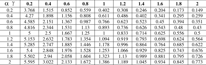 Table 1Page 3
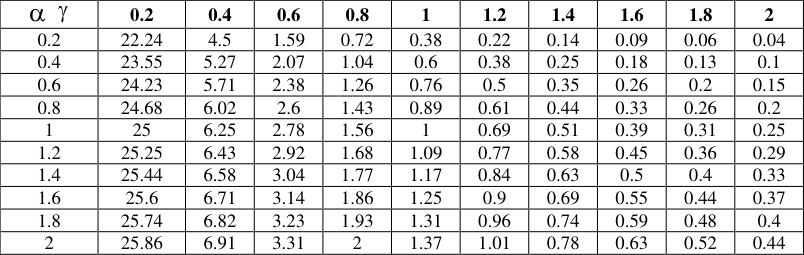 Table 1Page 3
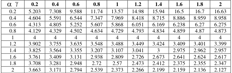 Table 1Page 3
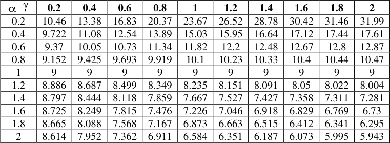 Table 1Page 4
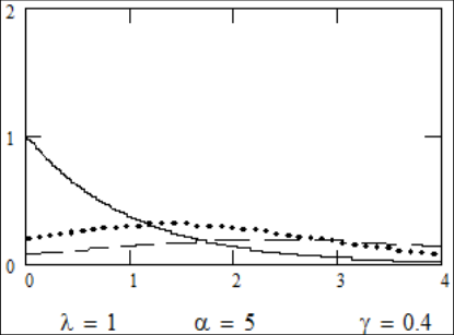 Figure 1Page 4
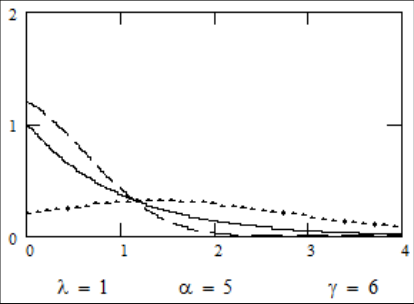 Figure 1Page 4
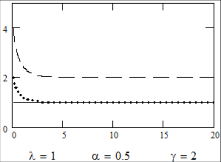 Figure 1Page 5
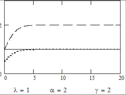 Figure 1Page 5
 Table 2Page 6
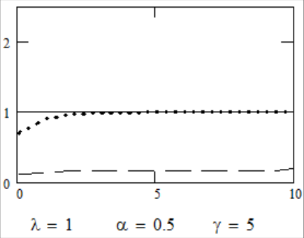 Figure 1Page 6
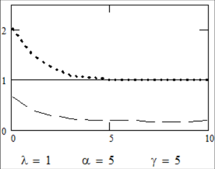 Figure 1Page 6
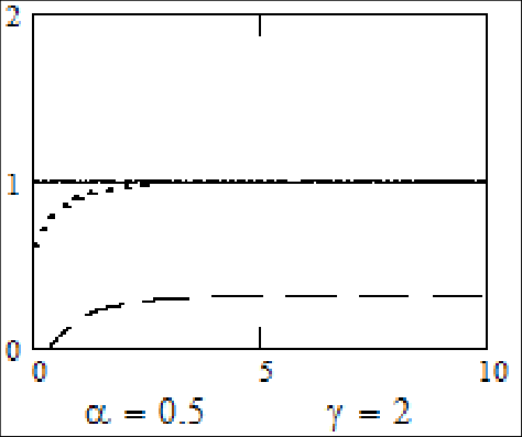 Figure 1Page 7
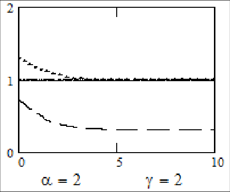 Figure 1Page 7
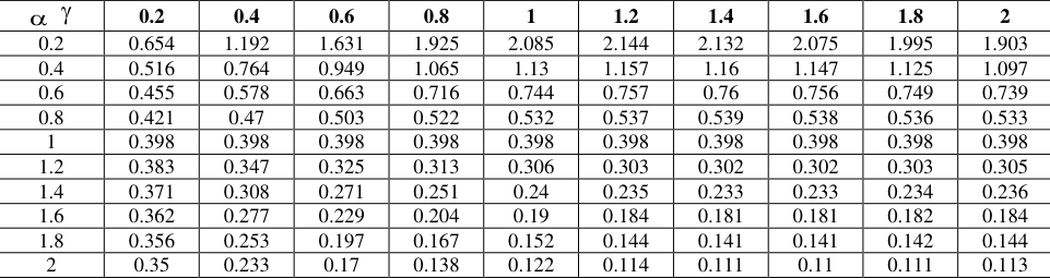 Table 2Page 10
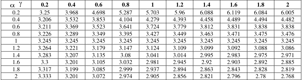 Table 2Page 10
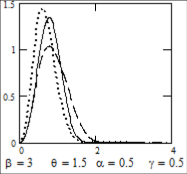 Figure 2Page 10
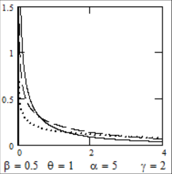 Figure 2Page 10
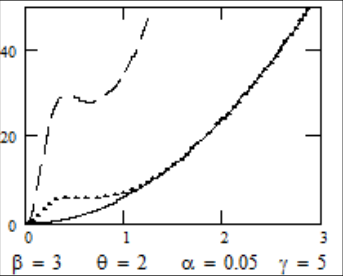 Figure 2Page 11
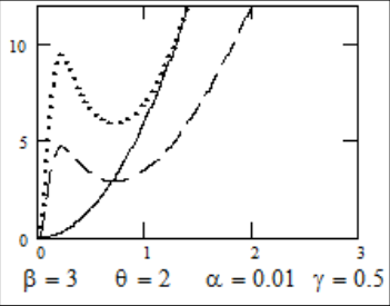 Figure 2Page 11
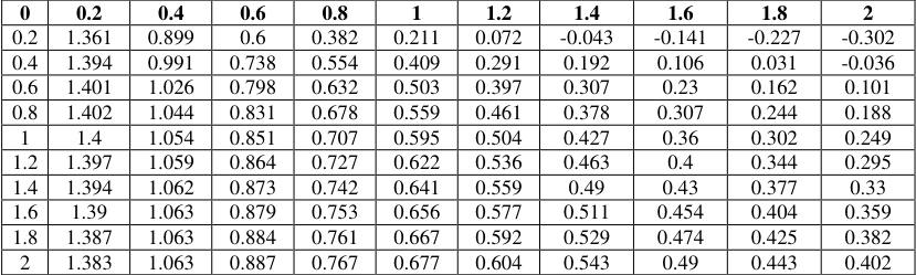 Table 2Page 12
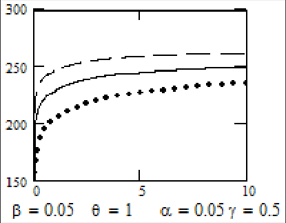 Figure 2Page 12
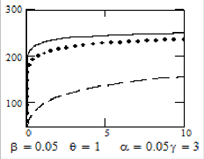 Figure 2Page 12
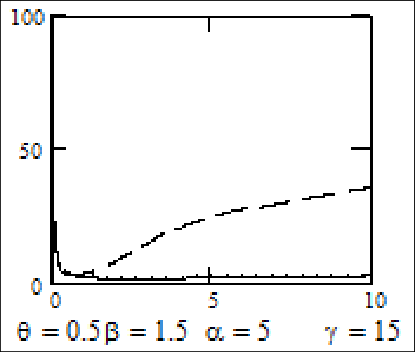 Figure 2Page 13
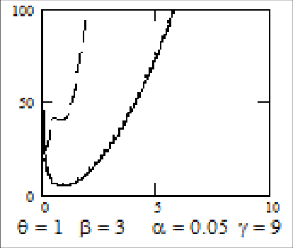 Figure 2Page 13
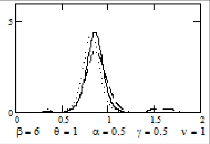 Figure 3Page 14
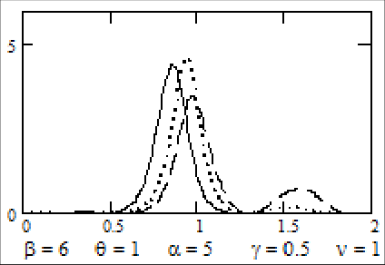 Figure 3Page 14
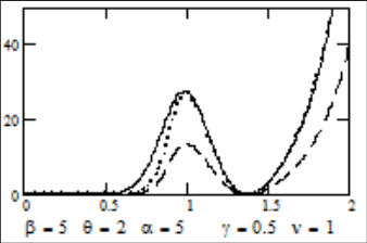 Figure 3Page 15
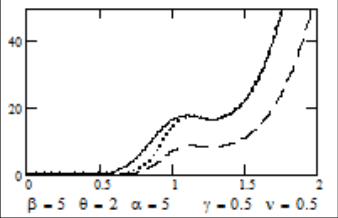 Figure 3Page 15
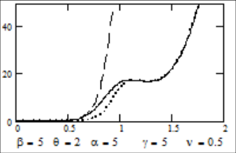 Figure 3Page 15
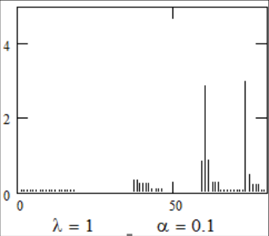 Figure 4Page 17
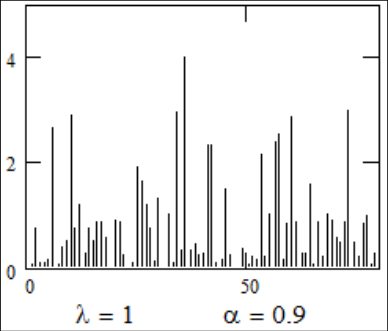 Figure 4Page 17
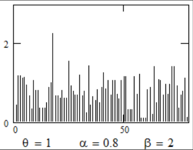 Figure 4Page 18
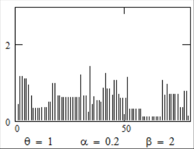 Figure 4Page 18
Introduction
Exponential distributions play a central role in analysis of lifetime or survival data, in part because of their convenient statistical theory, their important lack of memory property and their constant hazard rate. There are circumstances where the one-parameter family of exponential distributions is not sufficiently broad enough to represent lifetime data. A number of distributions like Gamma, Weibull, Gumble etc. are in common use. Here we shall introduce a general family of distributions, which includes exponential and Marshall-Olkin exponential distributions. A family of distributions containing both Weibull and Marshall-Olkin Weibull distributions are introduced and studied. Marshall and Olkin (1997) [26] introduced a method of adding parameters to distributions to expand families of distributions. This is a powerful method of adding parameters to a system of distributions. Sandhya and Prasanth (2014) [26] explained about Marshall-Olkin Discrete Uniform Distribution. Jayakumar and T.Mathew (2008) [15] generalized this method by adding one more parameter and applied it to Burr type XII distribution. Sandhya & Prasanth (2016) [27] detailed about a Generalized Discrete Uniform Distribution. They have illustrated some situations where this method is very useful. Throughout this paper, we refer to the Marshall-Olkin method as M-O method/scheme. The M-O scheme is as follows: Starting with a survival function F , the one-parameter family of survival functions
is called the M-O distribution generated from F . Marshall and Olkin (1997) [26] have applied this to exponential Weibull case. Jayakumar and T. Mathew (2008) [15] generalized this method and the two-parameter family of survival function , G is proposed as follows: , F(x) G (x)
x , 0 , 0 1 F(x) In Section 2, we study some of the properties of the three parameter exponential distribution, generated using our method described in (1.1). This three parameter exponential family has some nice properties. These properties are explored from reliability point of view. Weibull distribution is one of the common distributions applied in the field of communication engineering, reliability studies etc. These wide applications of the Weibull distribution have led to the further development in the theory of the distribution. A four parameter Weibull distribution using our method is the subject matter in Section 3. Several properties of this distribution from reliability practitioner's point of view are studied in this Section. Extension to semi-Weibull distribution is done in Section 4. Some of the interesting characteristics in the reliability point of view are also studied in this Section. The generalized semi-Weibull law is found to be of use in modeling data exhibiting periodic movements. Autoregressive time series modeling with non-Gaussian marginals is another area, which have attracted numerous researchers in recent years. This is based on the fact that many real data that we come across in practice are non-Gaussian in nature and usually skewed. We develop autoregressive models with distributions generated using M-O Scheme. Using this, one may be able to develop autoregressive processes with any given F as margnal. We also discuss the particular cases, MO exponential and MO Weibull autoregressive processes. These results are presented in Section 5.
A three parameter exponential family
Now consider the exponential family generated by (1.1). That is, in (1.1) when
The family of distributions with survival function , G will be referred to as the three-parameter exponential family in the sequel.
The density of the tree parameter exponential family is
The r th moment about zero is
The Tables given below gives the values of E(X) and V(X) for various values of , , for = 1. From Table 2.1, we can observe that for = 1 and = 1, E (X) = 1, as increases E (X) decreases and as increases E (X) increases. The same can be observed in the case of V (X) also. This phenomenon may be very useful in obtaining a variety of properties for the distribution for different values of and , which can be seen later in this article.
| 0 | 0.2 | 0.4 | 0.6 | 0.8 | 1 | 1.2 | 1.4 | 1.6 | 1.8 | 2 |
|---|---|---|---|---|---|---|---|---|---|---|
| 0.2 | 1.361 | 0.899 | 0.6 | 0.382 | 0.211 | 0.072 | -0.043 | -0.141 | -0.227 | -0.302 |
| 0.4 | 1.394 | 0.991 | 0.738 | 0.554 | 0.409 | 0.291 | 0.192 | 0.106 | 0.031 | -0.036 |
| 0.6 | 1.401 | 1.026 | 0.798 | 0.632 | 0.503 | 0.397 | 0.307 | 0.23 | 0.162 | 0.101 |
| 0.8 | 1.402 | 1.044 | 0.831 | 0.678 | 0.559 | 0.461 | 0.378 | 0.307 | 0.244 | 0.188 |
| 1 | 1.4 | 1.054 | 0.851 | 0.707 | 0.595 | 0.504 | 0.427 | 0.36 | 0.302 | 0.249 |
| 1.2 | 1.397 | 1.059 | 0.864 | 0.727 | 0.622 | 0.536 | 0.463 | 0.4 | 0.344 | 0.295 |
| 1.4 | 1.394 | 1.062 | 0.873 | 0.742 | 0.641 | 0.559 | 0.49 | 0.43 | 0.377 | 0.33 |
| 1.6 | 1.39 | 1.063 | 0.879 | 0.753 | 0.656 | 0.577 | 0.511 | 0.454 | 0.404 | 0.359 |
| 1.8 | 1.387 | 1.063 | 0.884 | 0.761 | 0.667 | 0.592 | 0.529 | 0.474 | 0.425 | 0.382 |
| 2 | 1.383 | 1.063 | 0.887 | 0.767 | 0.677 | 0.604 | 0.543 | 0.49 | 0.443 | 0.402 |
Table text extracted from the original PDF; superscript letters are shown inline. The original table image is below.
View original table image
| | 0.2 | 0.4 | 0.6 | 0.8 | 1 | 1.2 | 1.4 | 1.6 | 1.8 | 2 |
|---|---|---|---|---|---|---|---|---|---|---|
| 0.2 | 3.25 | 3.968 | 4.698 | 5.287 | 5.703 | 5.96 | 6.088 | 6.119 | 6.084 | 6.005 |
| 0.4 | 3.206 | 3.532 | 3.853 | 4.104 | 4.279 | 4.393 | 4.458 | 4.489 | 4.494 | 4.482 |
| 0.6 | 3.211 | 3.369 | 3.523 | 3.641 | 3.724 | 3.779 | 3.812 | 3.831 | 3.838 | 3.838 |
| 0.8 | 3.226 | 3.289 | 3.349 | 3.395 | 3.427 | 3.449 | 3.463 | 3.471 | 3.475 | 3.476 |
| 1 | 3.245 | 3.245 | 3.245 | 3.245 | 3.245 | 3.245 | 3.245 | 3.245 | 3.245 | 3.245 |
| 1.2 | 3.264 | 3.221 | 3.179 | 3.147 | 3.124 | 3.109 | 3.099 | 3.092 | 3.088 | 3.086 |
| 1.4 | 3.283 | 3.207 | 3.135 | 3.08 | 3.041 | 3.014 | 2.995 | 2.983 | 2.975 | 2.971 |
| 1.6 | 3.3 | 3.201 | 3.105 | 3.032 | 2.981 | 2.945 | 2.92 | 2.903 | 2.892 | 2.885 |
| 1.8 | 3.317 | 3.199 | 3.085 | 2.999 | 2.937 | 2.894 | 2.863 | 2.843 | 2.828 | 2.819 |
| 2 | 3.333 | 3.201 | 3.072 | 2.974 | 2.905 | 2.856 | 2.821 | 2.796 | 2.78 | 2.768 |
Table text extracted from the original PDF; superscript letters are shown inline. The original table image is below.
View original table image
| | 0.2 | 0.4 | 0.6 | 0.8 | 1 | 1.2 | 1.4 | 1.6 | 1.8 | 2 |
|---|---|---|---|---|---|---|---|---|---|---|
| 0.2 | 0.654 | 1.192 | 1.631 | 1.925 | 2.085 | 2.144 | 2.132 | 2.075 | 1.995 | 1.903 |
| 0.4 | 0.516 | 0.764 | 0.949 | 1.065 | 1.13 | 1.157 | 1.16 | 1.147 | 1.125 | 1.097 |
| 0.6 | 0.455 | 0.578 | 0.663 | 0.716 | 0.744 | 0.757 | 0.76 | 0.756 | 0.749 | 0.739 |
| 0.8 | 0.421 | 0.47 | 0.503 | 0.522 | 0.532 | 0.537 | 0.539 | 0.538 | 0.536 | 0.533 |
| 1 | 0.398 | 0.398 | 0.398 | 0.398 | 0.398 | 0.398 | 0.398 | 0.398 | 0.398 | 0.398 |
| 1.2 | 0.383 | 0.347 | 0.325 | 0.313 | 0.306 | 0.303 | 0.302 | 0.302 | 0.303 | 0.305 |
| 1.4 | 0.371 | 0.308 | 0.271 | 0.251 | 0.24 | 0.235 | 0.233 | 0.233 | 0.234 | 0.236 |
| 1.6 | 0.362 | 0.277 | 0.229 | 0.204 | 0.19 | 0.184 | 0.181 | 0.181 | 0.182 | 0.184 |
| 1.8 | 0.356 | 0.253 | 0.197 | 0.167 | 0.152 | 0.144 | 0.141 | 0.141 | 0.142 | 0.144 |
| 2 | 0.35 | 0.233 | 0.17 | 0.138 | 0.122 | 0.114 | 0.111 | 0.11 | 0.111 | 0.113 |
Table text extracted from the original PDF; superscript letters are shown inline. The original table image is below.
View original table image
| | 0.2 | 0.4 | 0.6 | 0.8 | 1 | 1.2 | 1.4 | 1.6 | 1.8 | 2 |
|---|---|---|---|---|---|---|---|---|---|---|
| 0.2 | 3.84 | 2.9 | 2.33 | 1.91 | 1.6 | 1.34 | 1.13 | 0.95 | 0.8 | 0.66 |
| 0.4 | 4.03 | 3.21 | 2.71 | 2.36 | 2.08 | 1.86 | 1.67 | 1.51 | 1.37 | 1.24 |
| 0.6 | 4.12 | 3.36 | 2.91 | 2.58 | 2.33 | 2.13 | 1.95 | 1.8 | 1.67 | 1.55 |
Table text extracted from the original PDF; superscript letters are shown inline. The original table image is below.
View original table image
The hazard rate exhibits both increasing and decreasing behavior. It can be seen that , r (x)
is increasing for 1 and is decreasing for 1.
this is also seen in the case of Marshall-Olkin exponential. But the rate of increase /decrease in hazard rate in the case of Marshall-Olkin exponential is far from our generalized exponential family. This can be seen from the Figure 1.2. A comparative study of the hazard rate functions of the exponential, Marshall-Olkin exponential and the new generalized scheme of exponential distribution with = 1 is presented in Figure 2. The solid lines represent the exponential distribution, dotted lines for Marshall-Olkin exponential and dashed lines for the general exponential distribution. We can observe that in the long run the general exponential distribution has constant hazard rate, which is a characteristic, observed in a number of real life situations. The mean residual life (MRL) has been used as far as the third century A.D. In the last two decades, however, reliability, statisticians and others have shown intensified interest in the MRL and derived many results concerning it. Given that a unit is of age t, the remaining life after time t is random. The expected value of this random residual life is called MRL at time t. A fascinating aspect about MRL is its tremendous range of applications. Actuaries apply MRL to setting rates and benefits for life insurance. In the biomedical setting researchers analyze survivorship studies by MRL. Increasing MRL distributions have been found useful as models in the social sciences for life lengths of wars and strikes (see Guess and Proschan, 1988) [13] . For any distribution F, the MRL is given by MRL (t)
In our situation this turns out to be
The integral is convergent but very tedious to workout. Numerical evaluation of the integral is possible using computers. A comparative study of the mean residual lifetime of the exponential, Marshall-Olkin exponential and generalized Marshall-Olkin exponential is given in Figure 1.3. The solid line represent exponential, doted line represents Marshall-Olkin exponential and dashed line represents the general exponential distributions. We can observe that in the long run the general exponential distribution has constant mean residual lifetime. One thing most engineers are agreed upon is that highly uncertain component or systems are inherently not realizable. But frequently they do not know how to measure the uncertainty. For example it is common practice among engineers that at the stage of designing a system, when there is enough information regarding the deterioration, wear of component parts, factors and levels are prepared based on this information. This type of information was usually obtained through hazard rate function or MRL function. How ever, in order to have a better design the stability of component parts should also be taken in to account together with the deterioration. For example, the better component is the component which lives longer and there is less uncertainty about its residual lifetime. The basic uncertainty measure for distribution F is differential entropy
dx. H is commonly refereed to as the Shannon's information measure. Intuitively speaking, H gives expected uncertainty contained in f(x) about the predictability an outcome of F. That is, H measures concentration of probabilities. Low entropy distributions are more concentrated, hence more informative that high entropy distributions (see Ebrahimi, 1996) [10] . In the case of our general family of distributions, the Shannon's measure of entropy is given by
The following table presents the Shannon's entropy measure of uncertainty of the general exponential family of distribution for various values of and with 0.2.
Note that there is less uncertainty for large values of and small values of . Also, for fixed , as increases, the uncertainty diminishes. Note that for fixed , as increases the uncertainty increases. Ebrahimi (1996) [10] introduced a modification to the Shannon's entropy measure. Frequently in survival analysis and life testing one has information about the current age of the component under consideration. In such cases, the age must be taken in to account when measuring uncertainty. Obliviously, the Shannon's entropy H is unsuitable in such situations and must be modified to take the age into account. A more realistic approach, which makes use of the age, is considered in Ebrahimi (1996) [10] . Given that a component has survived up to time t, the measure of entropy after time t given by
In the case of our exponential family, this is
The Figure 1.4. gives an idea about the distribution of modified Shannon's entropy about the values t = .5 and t = 5 with = 1.
From the Figures we can observe that the modified Shannon's entropy remains constant for large t. The cumulative distribution function G of a non negative random variable is said to be new better than used of specific age 0 t if 00 F(x t ) F(x)F(t ) and new worse than used when 00
F(x t ) F(x)F(t )
The general exponential distribution is new worse than used for 1 and new better than used if 1.
We can see that the 3 parameter general Marshall-Olkin exponential distribution give a variety of survival characteristics for various values of , and but preserves many of the characteristics of exponential distribution in the long run, and therefore will be very useful in reliability analysis, modeling etc….
A four-parameter weibull family
The Weibull distribution was first used to represent the distribution of breaking strength of materials and then for a wide variety of other applications (see Johnson et al. (1994). The Weibull distribution includes the exponential and Rayleigh distributions as special cases. It is well known that the hazard function of this distribution is a decreasing function when the shape parameter is less than 1, a constant when = 1 (exponential case), and increasing when >1. The use of the distribution in reliability and quality control work was advocated by many authors following Weibull (1951), Kao (1958, 1959), and Berrettoni (1964) [4] . Due to the nature of the hazard function described above, the distribution often become suitable where the conditions for strict "randomness" of the exponential distribution are not satisfied, with the shape parameter having a characteristic or predictable value depending upon the fundamental nature of the problem being considered. Unlike in the case of exponential distribution, probabilistic base for the Weibull distribution are not commonly encountered in situations where the distribution is actually employed. However, Malik (1975) [19] and Franck (1988) [12] have assigned some simple physical meanings and interpretations for the Weibull distribution, thus providing natural applications of this distribution in reliability problems particularly dealing with wearing styles. The distribution being a power transformation of the exponential, presents a convenient way of introducing some flexibility in the model through the power . Many authors have discussed the Weibull distribution in the analysis of wind speed. Pavia and O'Brien (1986) [22] used the Weibull distribution to model the wind speed over the ocean, while Carlin and Haslett (1982) [6] applied the distribution to model the wind power from a dispersed arrow of wind turbine generators. The Weibull distribution also found applications in analyzing rainfall and flood data, while Wilks (1989) [32] and Selker and Haith (1990) [28] applied the distribution to model rainfall intensity data. The Weibull model was utilized in many analyses relating to health science. For example, Berry (1975) [5] discussed the design of carcinogenesis experiments using the Weibull distribution. Dyer (1975) [8] applied the distribution to analyze the relationship of systolic blood pressure, serum cholesterol, and smoking to 14 year mortality in the Chicago Peoples Gas Company; coronary and cardiovascular-renal mortality were also compared in two competing risk models in the study. Whittemore and Altschuler (1976) used the model in the analysis of lung cancer incidence in cigarette smokers by considering Doll and Hills data for British Physician. Aitkin, Laird and Francis (1983) [1] applied the Weibull model in analyzing the Stanford heart transplant data. While carrying out a Bayesian analysis of survival curves for cancer patients following treatment, Chen et al. (1985) [7] utilized the Weibull distribution.
In addition to the above-mentioned application the Weibull distribution also found important use in a variety of other problems. For example, Fong, Rehm and Graminski (1977) [11] applied the distribution as a microscopic degradation model of paper. Weibull shelf life model for pharmaceutical problems was proposed by Ogden (1978) [21] . Rink et al. (1979) [25] used the three parameter Weibull distribution to quantify sweetgun germination data in genetic research. Application of Weibull distribution to the analysis of reaction time data has been introduced by Ida (1980) [14] . A role for the Weibull distribution in offshore oil/gas lease bidding problems has been demonstrated by Dyer (1981) [9] . The Weibull distribution is undeniably the distribution that has received maximum attention during the past decades. When
The r th moment of the distribution about zero is For some values of the parameter the hazard function is decreasing, for some other values the hazard rate is increasing and for some other values it exhibit non monotone characteristics. Also, unlike the usual Weibull law, this accounts a variety of changes in the ageing phenomena. This makes the distribution very rich in reliability characteristics.
The mean residual life (MRL) time is given by the equation
Event Hugh the expression is convergent It seems to be very tedious to evaluate it. But it is possible to find the values of the integral for various values of and . The table 3.3 present the Shannon's entropy measure of uncertainty of the general exponential family of distribution for various values of and with = 1 and = 2. The measure of entropy after time t given by Ebrahimi (1996) [10] is
The use of odds ratio and proportional odds is becoming more prevalent in engineering reliability and biological survival analysis when the data exhibit nonproportional hazards. However in some situations where the survival data indicate a nonmonotone hazard rate, the modeling by either proportional hazard or proportional odds may be lacking in their description of the situation. Wang et al. (2003) proposes the log odds rate (LOR) to characterize the distribution of failure, to provide a graphical examination of situations where the survival data indicate a non monotone hazard rate but monotone log odds rate, and further proposes the log odds rate as a new way of viewing and modeling the failure process in the region of aging.
The general semi Weibull distribution
A random variable X with positive support is said to follow semi-Weibull distribution if its survival function is given by (see Jose (1991) [24] . For example, P(X X )
<.5 we can estimate the value of by method of moments. Equate sample correlation to population correlation coefficient 1- and find the value of . Then the parameter can be estimated using the formula
where X is a random variable following Marshall-Olkin exponential distribution (see Marshall and Olkin (1997) [26] .
First Order Autoregressive Minification Process With Weibull Marginal Distribution
Consider the first order autoregressive minification process given by n n n 1 n w.p. X min(X , ) w.p. 1
where n is a sequence of independent and identically distributed random variables independent of {X n }. Then {X n } is stationary Markovian first order autoregressive Marshall-Olkin Weibull process with survival function H(x) if and only if n has Weibull distribution with survival function F(x) .
The proof and various properties can be established as above. Corr(X , X ) 1 .
. then we can conclude that the process is not a good fit. If We can estimate the value of by method of moments. Equate sample correlation to population correlation coefficient 1- and find the value of . Then the parameters and can be estimated using the integral formula for E(X r ) where X is a random variable following Marshall-Olkin Weibull distribution (see Marshall and Olkin (1997) [26] .
Figures and tables from the paper
| | 0.2 | 0.4 | 0.6 | 0.8 | 1 | 1.2 | 1.4 | 1.6 | 1.8 | 2 |
|---|---|---|---|---|---|---|---|---|---|---|
| 0.2 | 3.768 | 1.515 | 0.852 | 0.559 | 0.402 | 0.308 | 0.246 | 0.204 | 0.173 | 0.149 |
| 0.4 | 4.27 | 1.898 | 1.156 | 0.808 | 0.611 | 0.486 | 0.402 | 0.341 | 0.295 | 0.259 |
| 0.6 | 4.585 | 2.151 | 1.367 | 0.987 | 0.766 | 0.623 | 0.523 | 0.45 | 0.394 | 0.351 |
| 0.8 | 4.816 | 2.344 | 1.531 | 1.13 | 0.893 | 0.736 | 0.626 | 0.543 | 0.48 | 0.43 |
| 1 | 5 | 2.5 | 1.667 | 1.25 | 1 | 0.833 | 0.714 | 0.625 | 0.556 | 0.5 |
| 1.2 | 5.153 | 2.632 | 1.783 | 1.354 | 1.094 | 0.919 | 0.793 | 0.698 | 0.624 | 0.564 |
| 1.4 | 5.285 | 2.747 | 1.885 | 1.446 | 1.178 | 0.996 | 0.864 | 0.764 | 0.685 | 0.622 |
| 1.6 | 5.4 | 2.848 | 1.976 | 1.528 | 1.253 | 1.066 | 0.929 | 0.825 | 0.743 | 0.676 |
| 1.8 | 5.502 | 2.94 | 2.058 | 1.604 | 1.323 | 1.13 | 0.989 | 0.881 | 0.795 | 0.726 |
| 2 | 5.595 | 3.022 | 2.133 | 1.672 | 1.386 | 1.189 | 1.045 | 0.934 | 0.845 | 0.773 |
Table text extracted from the original PDF; superscript letters are shown inline. The original table image is below.
View original table image
| | 0.2 | 0.4 | 0.6 | 0.8 | 1 | 1.2 | 1.4 | 1.6 | 1.8 | 2 |
|---|---|---|---|---|---|---|---|---|---|---|
| 0.2 | 22.24 | 4.5 | 1.59 | 0.72 | 0.38 | 0.22 | 0.14 | 0.09 | 0.06 | 0.04 |
| 0.4 | 23.55 | 5.27 | 2.07 | 1.04 | 0.6 | 0.38 | 0.25 | 0.18 | 0.13 | 0.1 |
| 0.6 | 24.23 | 5.71 | 2.38 | 1.26 | 0.76 | 0.5 | 0.35 | 0.26 | 0.2 | 0.15 |
| 0.8 | 24.68 | 6.02 | 2.6 | 1.43 | 0.89 | 0.61 | 0.44 | 0.33 | 0.26 | 0.2 |
| 1 | 25 | 6.25 | 2.78 | 1.56 | 1 | 0.69 | 0.51 | 0.39 | 0.31 | 0.25 |
| 1.2 | 25.25 | 6.43 | 2.92 | 1.68 | 1.09 | 0.77 | 0.58 | 0.45 | 0.36 | 0.29 |
| 1.4 | 25.44 | 6.58 | 3.04 | 1.77 | 1.17 | 0.84 | 0.63 | 0.5 | 0.4 | 0.33 |
| 1.6 | 25.6 | 6.71 | 3.14 | 1.86 | 1.25 | 0.9 | 0.69 | 0.55 | 0.44 | 0.37 |
| 1.8 | 25.74 | 6.82 | 3.23 | 1.93 | 1.31 | 0.96 | 0.74 | 0.59 | 0.48 | 0.4 |
| 2 | 25.86 | 6.91 | 3.31 | 2 | 1.37 | 1.01 | 0.78 | 0.63 | 0.52 | 0.44 |
Table text extracted from the original PDF; superscript letters are shown inline. The original table image is below.
View original table image
| | 0.2 | 0.4 | 0.6 | 0.8 | 1 | 1.2 | 1.4 | 1.6 | 1.8 | 2 |
|---|---|---|---|---|---|---|---|---|---|---|
| 0.2 | 5.203 | 7.308 | 9.588 | 11.74 | 13.57 | 14.98 | 15.94 | 16.5 | 16.7 | 16.63 |
| 0.4 | 4.604 | 5.591 | 6.544 | 7.347 | 7.969 | 8.418 | 8.715 | 8.886 | 8.959 | 8.958 |
| 0.6 | 4.313 | 4.805 | 5.252 | 5.607 | 5.868 | 6.051 | 6.169 | 6.238 | 6.27 | 6.275 |
| 0.8 | 4.129 | 4.329 | 4.502 | 4.634 | 4.729 | 4.793 | 4.834 | 4.859 | 4.87 | 4.873 |
| 1 | 4 | 4 | 4 | 4 | 4 | 4 | 4 | 4 | 4 | 4 |
| 1.2 | 3.902 | 3.755 | 3.635 | 3.548 | 3.488 | 3.449 | 3.424 | 3.409 | 3.401 | 3.399 |
| 1.4 | 3.825 | 3.564 | 3.355 | 3.207 | 3.107 | 3.041 | 3 | 2.975 | 2.962 | 2.957 |
| 1.6 | 3.761 | 3.409 | 3.131 | 2.938 | 2.809 | 2.726 | 2.673 | 2.641 | 2.624 | 2.617 |
| 1.8 | 3.708 | 3.281 | 2.948 | 2.72 | 2.57 | 2.473 | 2.412 | 2.375 | 2.355 | 2.347 |
| 2 | 3.663 | 3.171 | 2.794 | 2.539 | 2.373 | 2.266 | 2.199 | 2.159 | 2.136 | 2.127 |
Table text extracted from the original PDF; superscript letters are shown inline. The original table image is below.
View original table image
| | 0.2 | 0.4 | 0.6 | 0.8 | 1 | 1.2 | 1.4 | 1.6 | 1.8 | 2 |
|---|---|---|---|---|---|---|---|---|---|---|
| 0.2 | 10.46 | 13.38 | 16.83 | 20.37 | 23.67 | 26.52 | 28.78 | 30.42 | 31.46 | 31.99 |
| 0.4 | 9.722 | 11.08 | 12.54 | 13.89 | 15.03 | 15.95 | 16.64 | 17.12 | 17.44 | 17.61 |
| 0.6 | 9.37 | 10.05 | 10.73 | 11.34 | 11.82 | 12.2 | 12.48 | 12.67 | 12.8 | 12.87 |
| 0.8 | 9.152 | 9.425 | 9.693 | 9.919 | 10.1 | 10.23 | 10.33 | 10.4 | 10.44 | 10.47 |
| 1 | 9 | 9 | 9 | 9 | 9 | 9 | 9 | 9 | 9 | 9 |
| 1.2 | 8.886 | 8.687 | 8.499 | 8.349 | 8.235 | 8.151 | 8.091 | 8.05 | 8.022 | 8.004 |
| 1.4 | 8.797 | 8.444 | 8.118 | 7.859 | 7.667 | 7.527 | 7.427 | 7.358 | 7.311 | 7.281 |
| 1.6 | 8.725 | 8.249 | 7.815 | 7.476 | 7.226 | 7.046 | 6.918 | 6.829 | 6.769 | 6.73 |
| 1.8 | 8.665 | 8.088 | 7.568 | 7.167 | 6.873 | 6.663 | 6.515 | 6.412 | 6.341 | 6.295 |
| 2 | 8.614 | 7.952 | 7.362 | 6.911 | 6.584 | 6.351 | 6.187 | 6.073 | 5.995 | 5.943 |
Table text extracted from the original PDF; superscript letters are shown inline. The original table image is below.
View original table image
References
33 in the original paper- Aitkin M, Laird N, Francis B. A reanalysis of Stanford heart transplant data (with discussion) Journal of American Statistical Association 1983;78:264-292.
- Arnold BC, Robertson CA. Autoregressive logistic process. Journal of Applied Probability 1989;26:524-531. Arnold BC. Logistic process involving Markovian minimization, 1993.
- Berrettoni JN. Practical applications of the Weibull distribution. Industrial Quality Control 1964;21:71-79.
- Berry G. Design of carcinogenesis experiments using the Weibull distribution, Biometrica 1975;62:321-328.
- Carlin J, Haslett J. Probability distribution of wind power from a dispersed array of wind turbine generators Jornal of Climate and Applied Metorology 1982;21:303-313.
- Chen WC, Hill BM, Greenhouse JB, Fayos JV. Bayesian analysis of survival curves for cancer patients following treatment, in Baysian Statistics, 2 Bernardo JM, DeGroot MH, Lindley DV, Smith AFM. (editors), 299-328, Amsterdam: NorthHolland. Communications in Statistics-Theory and Methods 1985;22:1649-1707.
- Dyer AR. An analysis of relationship of syatolic blood preasure, serum cholesterol, and smoking to 14-year mortality in the Chicago Peoples Gas Company study. Part I: Total mortality in exponential-Weibull model, Part II: Coronary and cardiovascular-renal mortality in two competing risk models Journal of Chronic Diseases 1975;28:565-578.
- Dyer D. Offshore oil/gas lease bidding and the Weibull distribution, In Statistical decisions in Scientific work, 6. Taillie GP, Patil, Baldessari BA. (editors), Dordrecht: Reidel, 1981, 33-45.
- Ebrahimi N. How to measure uncertainty in the residual life time distribution, 1996.
- Fong JT, Rehm RG, Graminski EL. Weibull statistics and a microscopic degradation model of paper Journal of the technical Association of the Pulp and paper Industry 1977;60:156-159.
- Franck JR. A simple explanation of Weibull distribution and its applications, 1988.
- Guess F, Proschan F. Mean residual life: Theory and Applications Hand Book of Statistics, Elsevier Science Publishers, B.V 1988;7:215-224.
- Ida M. The application of the Weibull distribution to the analysis of the reaction time data, Japanice Phychological Research IEE transactions on Reliability 1980;22:207-212.
- Jayakumar K, Thomas Mathew. On a generalization to Marshall-Olkin Scheme and its application to Burr type XII distribution Statistical Papers 2008;49:421-439.
- Kao JHK. Computer methods for estimating Weibull parameters in reliability studies. Transactions of IRE-Reliability and Quality Control 1958;13:397-404.
- Kao JHK. A graphical estimation of mixed Weibull parameters in life testing electron tubes, Technometrics 1959;1:389-407.
- Lewis PAW, McKenzie Ed. Minification processes and their transformations. Journal of Applied Probability 1991;28:45-57.
- Malik MAK. A note on the physical meaning of the Weibull distribution, 1975.
- Marshall AW, Olkin I. A new method for adding a parameter to a family of distributions with applications to exponential and Weibull families Biometrika 1997;84:641-652.
- Ogden JE. A Weibull shelf-life model for Pharmaceutical ASQC Technical Conference Transactions 1978, 574-580.
- Pavia EJ, O'Brien JJ. Weibull statistics of the wind speed over the ocean, 1986.
- Pillai RN. Semi-Pareto processes. Journal of Applied Probability 1991;28:461-465.
- Pillai RN, Jose KK, Jayakumar K. Autoregressive minification processes & class of universal geometrical minima. Journal of Indian Statistical Association 1995;33:53-61.
- Rink G, Dell TR, Swizer G, Bonner FT. Use of the [three parameter] Weibull function to quantifysweetgun germinating data Silvae genetica 1979;28:9-12.
- Sandhya E, Prasanth CB. Marshall-Olkin Discrete Uniform Distribution, Journal of Probability, Hindawi Publishing Corporations, 2014, 10. http://dx.doi.org/10.1155/2014/979312,
- Sandhya E, Prasanth CB. A Generalized Discrete Uniform Distribution, Journal of Statistics Applications & Probability, An International Journal, Natural Sciences Publishing (NSP) 2016. doi:10.18576/jsap/050110
- Selker JS, Haith DA. Development and testing of single parameter precipitation distribution, 1990.
- Sim CH. Simulation of Weibull and Gamma Autoregressive Stationary Processes. Communications in Statistics -Simulation and Computation 1986;15:1141-1146.
- Weibull W. A Statistical distribution of wide applicability Journal of Applied Mechanics 1951;18:293-297.
- Whittemore A, Altschuler B. Lung cancer incedence in cigarate smokers: Further analysis for Doll and Hill's data foe Britsh Physicians, Biometrics 1976;32:805-816.
- Wilks DS. Rainfall intessity, the Weibull distribution, and estimation of daily surface runoff Journal of Applied Meterology 1989;28:52-58.
- Yao Wang, Hossain AM, Zimmer WJ. Monotone Log-Odds Rate Distributions in Reliability Analysis Communications in Statistics-Theory and Methods 2003;32:2227-2244.
- Yeh HC, Arnold BC, Robertson CA. Pareto processes. Journal of Applied Probability 1988;25:291-301.