
Research article · 2020 · Full text
International Journal of Statistics and Applied MathematicsLindley Gompertz distribution with properties and applications
Volume 5(6) · Pages 28–37 · DOI: 10.22271/maths.2020.v5.i6a.610 ↗
Research areasStatistical Distribution Estimation and ApplicationsBayesian Methods and Mixture ModelsStatistical Methods and Bayesian Inference
Abstract
Author-writtenIn this article, we have presented a new three-parameter probability distribution called the Lindley Gompertz distribution. The proposed model can exhibit increasing, increasing-decreasing, j-shaped, and bathtub, and a broad variety of monotone failure rates. Some properties of this model are studied and calculated. Three extensively used estimation methods are used to estimate the model parameters namely maximum likelihood estimators (MLE), least-square (LSE), and Cramer-Von-Mises (CVM) methods. By using the maximum likelihood estimate we have constructed the asymptotic confidence interval for the model parameters. All the computations are performed in R software. The potentiality of the proposed distribution is revealed by using some graphical methods and statistical tests taking a real dataset, where the proposed distribution provided a better fit and more flexible in comparison with some other lifetime distributions.
Summary
Source-checkedPlain-language reading of the full paper, prepared with AI and checked against the text. Each point links to the authors' own words.
Why it matters
- Existing continuous probability distributions often fail to provide an adequate fit for real-world datasets across various fields such as life sciences, engineering, and risk analysis. View evidence ↗
- Creating modified distributions by adding parameters or transforming baseline distributions can result in models that are more flexible and provide a better fit for data. View evidence ↗
- The Gompertz distribution is a classical model used significantly for analyzing actuarial tables and human mortality based on survival functions. View evidence ↗
The question
- The authors aim to introduce a new three-parameter probability distribution known as the Lindley Gompertz (LG) distribution. View evidence ↗
- The study is motivated by the goal of increasing the flexibility of the Gompertz distribution to better fit real data by adding a single extra parameter. View evidence ↗
What they did
- The model parameters are estimated using three common methods: maximum likelihood estimators (MLE), least-square (LSE), and Cramer-Von-Mises (CVM). View evidence ↗
- To test the distribution, the authors used a real dataset consisting of failure times from an accelerated life test of 59 microcircuit conductors. View evidence ↗
- All statistical computations for the study were carried out using R software. View evidence ↗
What they found
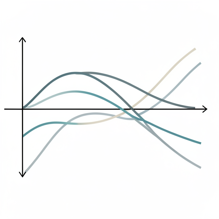
- The LG distribution is capable of exhibiting a wide variety of failure rates, including bathtub, j-shaped, increasing, increasing-decreasing, and monotone rates. View evidence ↗
- Using MLE on the conductor dataset, the estimated parameters were alpha = 0.1765, lambda = 0.2051, and theta = 11.4574. View evidence ↗
- Comparing estimation methods, MLE yielded the lowest negative log-likelihood (111.8046) and the lowest AIC (229.6092) compared to LSE and CVE. View evidence ↗
- The LG distribution showed a better fit than competing models (FW, LE, EP, GZ), exhibiting the minimum KS (0.0620), W (0.0331), and A2M (0.1988) statistics. View evidence ↗
- In terms of information criteria, the LG model had a lower negative log-likelihood (111.8046) than the LE (114.9528), EP (116.5015), and GZ (117.1740) models. View evidence ↗
What it means
- The authors conclude that the maximum likelihood estimation (MLE) is the superior method for estimating parameters compared to LSE and CVM. View evidence ↗
- The authors state that the LG model is more flexible and provides a consistently better fit than other models, suggesting it will be useful for survival analysis. View evidence ↗
Visual summary
3 visualsIllustrations explain the paper; charts are replotted from the paper's own table values.
Hazard Function Versatility
AI-generated conceptual illustration (mathematical probability curves on a coordinate plane). It explains the idea and does not show study data.
View source evidence ↗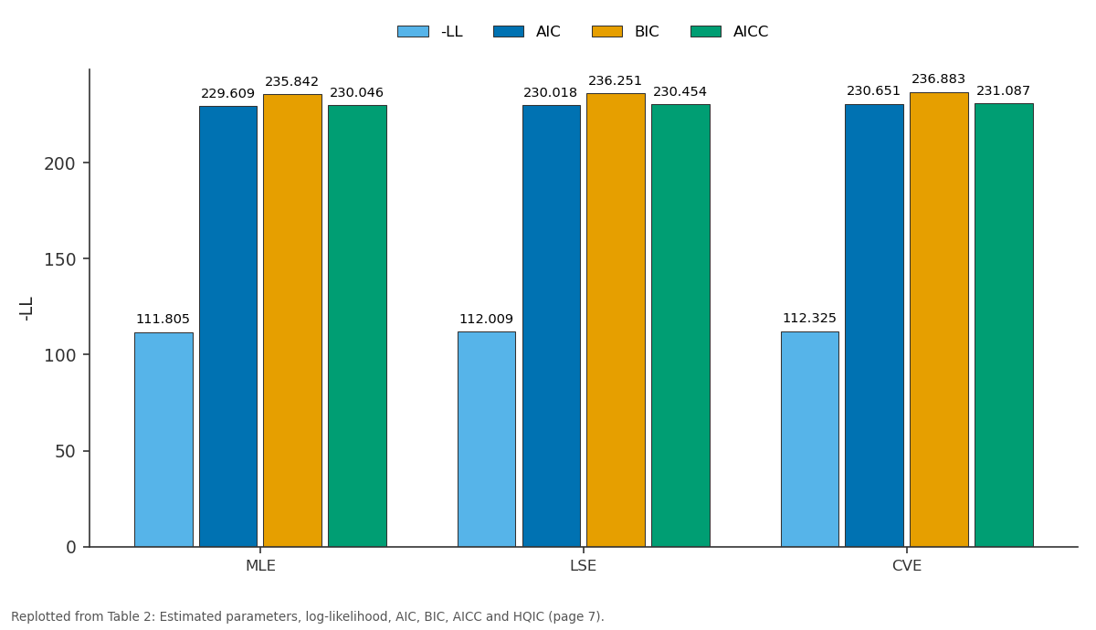
-LL and AIC and more: MLE vs LSE vs CVE
Replotted from Table 2 (page 7) of the original paper. Every bar is the paper's own table value.
View source evidence ↗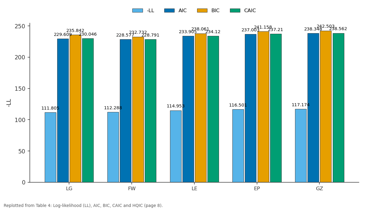
-LL and AIC and more: LG vs FW vs LE vs EP vs GZ
Replotted from Table 4 (page 8) of the original paper. Every bar is the paper's own table value.
View source evidence ↗Figures & tables
From the original paper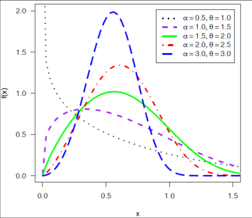 Figure 1
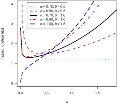 Figure 1
 Table 1
 Table 2
 Table 3
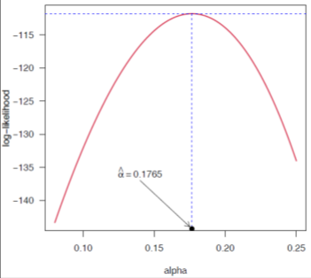 Figure 2
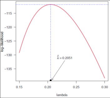 Figure 2
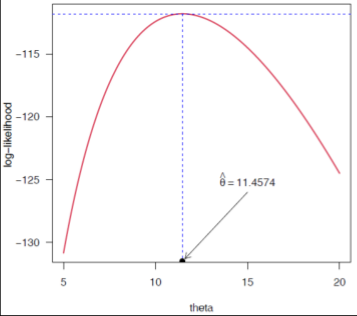 Figure 2
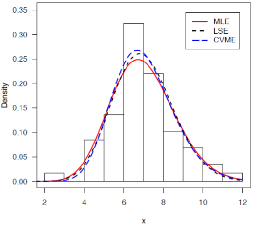 Figure 3
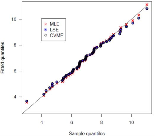 Figure 3
 Table 4
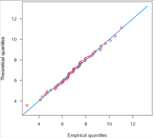 Figure 4
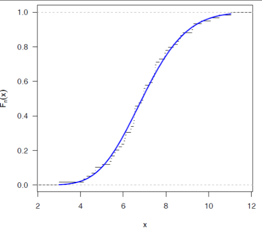 Figure 4
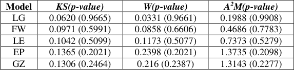 Table 5
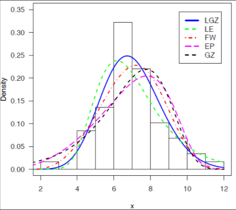 Figure 5
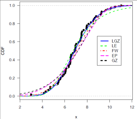 Figure 5
Introduction
Most of the continuous probability distributions have been introduced in recent years but the real data sets related to life sciences, engineering, finance, climatology, medicine, geology, biology, hydrology, ecology, reliability, life testing, and risk analysis do not provide a better fit to these distributions. So, the creation of new modified distributions seems to be necessary to address the problems in these fields. The generalized, extended, and modified distributions are created by adding one or more parameters or performing some transformations to the baseline distribution. Therefore, the new proposed distributions provide the best fit and more flexible compared to the competing models. Researchers in the last few decades have developed various extensions and a modified form of the Lindley distribution which was developed by (Lindley, 1958) [19] in the context of Bayesian statistics, as a counterexample to fiducial statistics. An extensive study on the Lindley distribution was done by (Ghitany et al., 2008) [11] , Mazucheli & Achcar (2011) [21] have been used the Lindley distribution to competing risks lifetime data. A random variable X follows Lindley distribution with parameter θ and its probability density function (PDF) is given by
And its cumulative density function (CDF) is
In this article, we put forward the new Lindley Gompertz (LG) distribution to enhance the capability of the Lindley distribution using the Lindley-G family by inserting only one extra parameter. It is a member of the Lindley-G family introduced by Ristic and Balakrishnan (2012) [27] .
Here, we have taken the Lindley distribution as a generator and the Gompertz as a baseline distribution. Towards the modified theoretical distribution, Ghitany et al. (2011) [12] introduced weighted Lindley distribution having two parameters and has shown that it is appropriate in modeling survival data for a mortality study. Nadarajah et al. (2011) [24] have introduced generalized Lindley, extended Lindley by (Bakouch et al., 2012) [4] , Ashour and Eltehiwy (2015) [3] for exponentiated power Lindley, Bhati et al. (2015) [5] Lindley-Exponential distribution. Ieren et al. (2018) [15] have introduced modeling lifetime data with Weibull-Lindley distribution. Ibrahim et al. (2019) [14] has introduced a new extension of Lindley distribution. Alizadeh et al. (2020) [2] have introduced the odd log-logistic Lindley-G family of distributions and illustrated the Bayesian and non-Bayesian estimation of the model parameter. Cakmakyapan and Ozel (2016) [7] have presented a new class of distributions to generate new distribution based on the Lindley generator (Lindley-G) having additional shape parameter θ. The CDF and PDF of Lindley-G are respectively,
The Gompertz distribution is one of the classical probability distribution that represents survival function based on laws of mortality. This distribution performs a significant role in modeling human mortality and analyzing actuarial tables. The Gompertz distribution was first introduced by (Gompertz, 1824) [13] . It has been used as a growth model and also used to fit the tumor growth. The Gompertz function reduced a significant collection of data in life tables into a single function. It is based on the assumption that the mortality rate decreases exponentially as a person ages. The resulting Gompertz function is for the number of individuals living at a given age as a function of age. Applications and an extensive survey of the Gompertz distribution can be found in (Ahuja & Nash, 1967) [1] . Cooray and Ananda (2010) [9] have introduced the Gompertz-sinh family and it was used to analyze the survival data with highly negatively skewed distribution. El-Gohary et al. (2013) [10] have presented a flexible called the generalized Gompertz distribution it has increasing or constant or decreasing or bathtub curve failure rate depending upon the shape parameter. Ieren et al. (2019) [16] have introduced a three-parameter power Gompertz distribution using a power transformation approach. The motivation of this study is to obtain a more flexible model by adding just one extra parameter to the Gompertz distribution to achieve a better fit to the real data. We study the properties of the LG distribution and explore its applicability. The contents of this article are organized as follows. The new Gompertz distribution is introduced and various distributional properties are discussed in Section 2. Three commonly used estimation methods are employed to estimate the model parameters namely maximum likelihood estimators (MLE), least-square (LSE) and Cramer-Von-Mises (CVM) methods, further, the maximum likelihood estimators are used to construct the asymptotic confidence intervals using the observed information matrix is discussed in Section 3. In Section 4 a real data sets have been taken to investigate the applications and suitability of the proposed distribution. In this section, we present the ML estimators of the parameters and approximate confidence intervals also AIC, BIC, AICC, HQIC are calculated to assess the validity of the LG model. Finally, Section 5 ends up with some general concluding remarks.
The Lindley Gompertz distribution
The Gompertz distribution was first introduced by (Gompertz, 1824) [13] . Let X be a random variable follows the Gompertz distribution with parameters α and λ if its cumulative distribution function can be written as,
and its corresponding probability density function can be expressed as,
Using ( 5) and ( 6) as CDF and PDF of baseline distribution to (3) and ( 4) we get the CDF and PDF of Lindley Gompertz distribution with parameters , , 0
Reliability/survival function
The reliability function of Lindley Gompertz (LG) distribution is
Hazard function
The failure rate function of LG distribution can be defined as,
Quantile function
The quantile function of LG (α, λ, θ) can be expressed as,
The Random Deviate Generation:
The random deviate can be generated from LG (α, λ, θ) by
Solving ( 12) for x we get the expression for the random deviate generation; here v has the U (0, 1) distribution. Plots of probability density function and hazard rate function of LG (α, λ, θ) with different values of parameters are shown in Figure 1.
Skewness and Kurtosis of LG distribution:
In descriptive statistics, the measures of skewness and kurtosis play a significant role in data analysis. The coefficient of Bowley's skewness measure based on quartiles is given by
and the coefficient of Moor's kurtosis measures based on octiles Moors (1988) is given by
Methods of Estimation
The objective of estimation is to approximate the value of a model parameter based on sample information. The estimation theory deals with the basic problem of inferring some relevant features of a random experiment based on the observation of the experiment outcomes. There are so many methods for estimating unknown parameters of the model. We have considered three types of estimation methods such as the maximum likelihood (MLE), ordinary least squares (LSE), and the Cramer-von Mises (CVM) method.
Maximum Likelihood Estimation (MLE)
We have illustrated the maximum likelihood estimators (MLE's) of the LG (α, λ, θ) distribution. Let x̠ = (x1,…..,xn) be the observed values of size 'n' from LG (α, λ, θ) then the likelihood function for the parameter vector
taking logarithms on both sides we get
The elements of the score function
The observed fisher information matrix  as an estimate of the information matrix
here H is the Hessian matrix.
The Newton-Raphson algorithm to maximize the likelihood produces the observed information matrix. Therefore, the variancecovariance matrix is given by,
Hence from the asymptotic normality of MLEs, approximate 100(1-α) % confidence intervals for α, λ, and θ can be constructed as, Z is the upper percentile of standard normal variate.
Method of Least-Square Estimation (LSE)
The ordinary least square estimators and weighted least square estimators are introduced by (Swain et al., 1988) [26] to estimate the parameters of Beta distributions. The least-square estimators of the unknown parameters for α, λ, and θ of LG distribution can be obtained by minimizing
X ,X , .., X is a random sample of size n from a (2.3). Therefore, the least square estimators of α, λ, and θ say ˆ, and
respectively, can be obtained by minimizing
, , 1 e x p 1 e x p 1 lo g 1 e x p 1 e x p 1 1 1
with respect to α, λ, and θ.
To obtain the least square estimates of α, λ, and θ, we have to solve the following two nonlinear equations simultaneously by equating to zero,
Method of Cramer-Von-Mises (CVM)
We are interested in Cramér-von-Mises type minimum distance estimators, (Macdonald 1971) [20] because it provides empirical evidence that the bias of the estimator is smaller than the other minimum distance estimators. The CVM estimators of α, λ, and θ are obtained by minimizing the function
To obtain the CVM estimators of α, λ, and θ, we have to solve the following two nonlinear equations simultaneously by equating to zero.
Application with a real dataset
In this section, we illustrate the applicability of LIW distribution using a real dataset used by earlier researchers. Lawless (2003) [18] failures can occur in microcircuits because of the movement of atoms in the conductors in the circuit; this is referred to as electromigration. The data below are from an accelerated life test of 59 conductors. Failure times are in hours and there are no censored observations. The maximum likelihood estimates are calculated directly by using optim() function in R software (R Core Team, 2020) [27] and (Ming Hui, 2019) [22] by maximizing the likelihood function (3.1). We have obtained = 0.1765, = 0.2051, = 11.4574 and corresponding Log-Likelihood value is -111.8046. In Table 1 we have demonstrated the MLE's with their standard errors (SE) and 95% confidence interval for α, λ, and θ. The plots of profile log-likelihood function (Kumar & Ligges, 2011) [17] for the parameters α, λ and θ have been displayed in Figure 2 and noticed that the ML estimates can be uniquely determined. In Table 2 we have displayed the estimated value of the parameters of Lindley Gompertz distribution using MLE, LSE and CVE method and their corresponding negative log-likelihood, AIC, BIC, AICC and HQIC criterion. In Table 3 we have presented The KS, W and A 2 statistics with their corresponding p-value of MLE, LSE and CVE method. To illustrate the goodness of fit of the Lindley Gompertz distribution, we have taken some well-known distribution for comparison purpose which are listed blew,
| Method of Estimation | KS(p-value) | W(p-value) | A2M(p-value) |
|---|---|---|---|
| MLE | 0.0620(0.9665) | 0.0331(0.9661) | 0.1988(0.9908) |
| LSE | 0.0553(0.9893) | 0.0273(0.9848) | 0.2125(0.9866) |
| CVE | 0.0516(0.9953) | 0.0256(0.9890) | 0.2457(0.9726) |
Table text extracted from the original PDF; superscript letters are shown inline. The original table image is below.
View original table image
| Method of Estimation | ˆ | ˆ | ˆ | -LL | AIC | BIC | AICC | HQIC |
|---|---|---|---|---|---|---|---|---|
| MLE | 0.17654 | 0.20507 | 11.4574 | 111.8046 | 229.6092 | 235.8418 | 230.0455 | 232.0421 |
| LSE | 0.20892 | 0.17088 | 10.37019 | 112.0091 | 230.0182 | 236.2508 | 230.4545 | 232.4511 |
| CVE | 0.15321 | 0.26034 | 17.3537 | 112.3254 | 230.6508 | 236.8834 | 231.0872 | 233.0838 |
Table text extracted from the original PDF; superscript letters are shown inline. The original table image is below.
View original table image
| Parameter | MLE | SE | 95% ACI |
|---|---|---|---|
| alpha | 0.1765 | 0.0466 | (0.0853, 0.2678) |
| lambda | 0.2051 | 0.0594 | (0.0887, 0.3215) |
| theta | 11.4574 | 3.1947 | (5.1959, 17.7189) |
Table text extracted from the original PDF; superscript letters are shown inline. The original table image is below.
View original table image
Flexible Weibull Extension (FWE) distribution
The density of Flexible Weibull (FW) distribution (Bebbington, 2007) [5] with parameters α and β is 2 ( ) e x p e x p e x p ; 0 , 0 , 0 .
Lindley-Exponential (LE) distribution
The probability density function of LE (Bhati, 2015) [6] can be expressed as
Exponential power (EP) distribution
The probability density function Exponential power (EP) distribution (Smith & Bain, 1975) [25] is
. where α and λ are the shape and scale parameters, respectively.
Gompertz distribution (GZ)
The probability density function of Gompertz distribution (Murthy et al., 2003) [23] with parameters α and θ is
In Figure 4 we have plotted the Q-Q plot and CDF plot and it is seen that the proposed distribution fits the data very well. For the assessment of potentiality of the proposed model we have calculated the Akaike information criterion (AIC), Bayesian information criterion (BIC), Corrected Akaike information criterion (CAIC) and Hannan-Quinn information criterion (HQIC) which are presented in Table 4. The Histogram and the density function of fitted distributions and Empirical distribution function with the estimated distribution function of LG and some selected distributions are presented in Figure 5. To compare the goodness-of-fit of the LG distribution with other competing distributions we have presented the value of Kolmogorov-Simnorov (KS), the Anderson-Darling (W) and the Cramer-Von Mises (A 2 ) statistics in Table 5. It is observed that the LG distribution has the minimum value of the test statistic and higher p-value thus we conclude that the LG distribution gets quite better fit and more consistent and reliable results from others taken for comparison.
| Model | KS(p-value) | W(p-value) | A2M(p-value) |
|---|---|---|---|
| LG | 0.0620 (0.9665) | 0.0331 (0.9661) | 0.1988 (0.9908) |
| FW | 0.0971 (0.5991) | 0.0858 (0.6606) | 0.4686 (0.7783) |
| LE | 0.1042 (0.5099) | 0.1173 (0.5077) | 0.7373 (0.5279) |
| EP | 0.1365 (0.2021) | 0.2398 (0.2021) | 1.3735 (0.2098) |
| GZ | 0.1306 (0.2464) | 0.216 (0.2387) | 1.3143 (0.2277) |
Table text extracted from the original PDF; superscript letters are shown inline. The original table image is below.
View original table image
| Model | -LL | AIC | BIC | CAIC | HQIC |
|---|---|---|---|---|---|
| LG | 111.8046 | 229.6092 | 235.8418 | 230.0455 | 232.0421 |
| FW | 112.2883 | 228.5766 | 232.7317 | 228.7909 | 230.1986 |
| LE | 114.9528 | 233.9055 | 238.0606 | 234.1198 | 235.5275 |
| EP | 116.5015 | 237.0029 | 241.1580 | 237.2098 | 238.6249 |
| GZ | 117.1740 | 238.3480 | 242.5031 | 238.5623 | 239.9700 |
Table text extracted from the original PDF; superscript letters are shown inline. The original table image is below.
View original table image
Conclusion
In this article, we have developed the three-parameter continuous Lindley Gompertz (LG) distribution. For our study, we have provided the statistical and mathematical properties of the proposed model. The shape of the PDF of the LG model is uni-modal and positively skewed and the hazard function can exhibit increasing, increasing-decreasing, j-shaped and bathtub, and a broad variety of monotone failure rates. The P-P and KS plots showed that the purposed distribution is quite better for fitting the real dataset. Finally, using a real data set we have explored some well-known estimation methods namely maximum likelihood estimation (MLE), least-square (LSE), and Cramer-Von-Mises (CVM) methods. Further, we also construct the asymptotic confidence interval for MLEs. We conclude that MLE is the best estimation method as compared to the LSE and CVM methods. The application illustrates that the proposed model provides a consistently better fit and more flexible than other underling models. We expect that this model will contribute to the field of survival analysis.
Figures and tables from the paper
References
28 in the original paper- Ahuja JC, Nash SW. The generalized Gompertz-Verhulst family of distributions. Sankhyā: The Indian Journal of Statistics, Series A. 1967; 1:141-56.
- Alizadeh M, Afify AZ, Eliwa MS, Ali S. The odd log-logistic Lindley-G family of distributions: properties, Bayesian and non-Bayesian estimation with applications. Computational Statistics. 2020; 35(1):281-308.
- Ashour SK, Eltehiwy MA. Exponentiated power Lindley distribution. Journal of advanced research. 2015; 6(6):895-905.
- Ashour SK, Eltehiwy MA. Exponentiated power Lindley distribution. Journal of advanced research. 2015; 6(6):895-905.
- Bebbington M, Lai CD, Zitikis R. A flexible Weibull extension. Reliability Engineering & System Safety. 2007; 92(6):71926.
- Bhati D, Malik MA, Vaman HJ. Lindley-Exponential distribution: properties and applications. Metron. 2015; 73(3):335-57.
- Cakmakyapan S, Gamze OZ. The Lindley family of distributions: Properties and applications. Hacettepe Journal of Mathematics and Statistics. 2016; 46(6):1113-37.
- Casella G, Berger RL. Statistical Inference. Brooks. Cole Publishing, CADenux T, Masson MH, Hbert PA (2005) Nonparametric rank-based statistics and significance tests for fuzzy data. Fuzzy Sets Syst. 1990; 153:128Dubois.
- Cooray K, Ananda MM. Analyzing survival data with highly negatively skewed distribution: The Gompertz-sinh family. Journal of Applied Statistics. 2010; 37(1):1-1.
- El-Gohary A, Alshamrani A, Al-Otaibi AN. The generalized Gompertz distribution. Applied Mathematical Modelling. 2013; 37(1-2):13-24.
- Ghitany ME, Atieh B, Nadarajah S. Lindley distribution and its application. Mathematics and computers in simulation. 2008; 78(4):493-506.
- Ghitany ME, Alqallaf F, Al-Mutairi DK, Husain HA. A two-parameter weighted Lindley distribution and its applications to survival data. Mathematics and Computers in simulation. 2011; 81(6):1190-201.
- Gompertz, B. On the nature of the function expressive of the law of human mortality and on the new mode of determining the value of life contingencies. Phil. Trans. Royal Soc. A. 1824; 115:513-580.
- Ibrahim M, Yadav AS, Yousof HM, Goual H, Hamedani GG. A new extension of Lindley distribution: modified validation test, characterizations and different methods of estimation. Communications for Statistical Applications and Methods. 2019; 26(5):473-95.
- Ieren TG, Oyamakin SO, Chukwu AU. Modeling lifetime data with Weibull-Lindley distribution. Biometrics and Biostatistics International Journal. 2018; 7(6):532-44.
- Ieren TG, Kromtit FM, Agbor BU, Eraikhuemen IB, Koleoso PO. A power Gompertz distribution: Model, properties and application to bladder cancer data. Asian Research Journal of Mathematics. 2019; 19:1-4.
- Kumar V, Ligges U. reliaR: A package for some probability distributions, 2011. http://cran.rproject.org/web/packages/reliaR/index.html.
- Lawless JF. Statistical models and methods for lifetime data. John Wiley & Sons; 2011 Jan 25.
- Lindley, DV. Fiducial distributions and Bayes' theorem, Journal of the Royal Statistical Society Series B. 1958; 20:102-107.
- Macdonald PD. Comments and Queries Comment on "An Estimation Procedure for Mixtures of Distributions" by Choi and Bulgren. Journal of the Royal Statistical Society: Series B (Methodological). 1971; 33(2):326-9.
- Mazucheli J, Achcar JA. The Lindley distribution applied to competing risks lifetime data. Computer methods and programs in biomedicine. 2011; 104(2):188-92.
- Hui EG, Hui EG, John S. Learn R for Applied Statistics. Apress, 2019.
- Murthy DNP, Xie M, Jiang R. Weibull Models, Wiley, New York, 2003.
- Nadarajah S, Bakouch HS, Tahmasbi R. A generalized Lindley distribution. Sankhya B. 2011; 73(2):331-59.
- Smith RM, Bain LJ. An exponential power life-test distribution, Communications in Statistics. 1975; 4:469-481.
- Swain JJ, Venkatraman S, Wilson JR. Least-squares estimation of distribution functions in Johnson's translation system. Journal of Statistical Computation and Simulation. 1988; 29(4):271-97.
- R Core Team. R: A language and environment for statistical computing. R Foundation for Statistical Computing, 2020, Vienna, Austria. URL https://www.R-project.org/.
- Ristić MM, Balakrishnan N. The gamma-exponentiated exponential distribution. Journal of Statistical Computation and Simulation. 2012; 82(8):1191-206.
Cited by 7
From OpenAlex, OpenCitations and reference lists read by Scinovex
- The entropy-transformed Gompertz distribution: Distributional insights and cross-disciplinary utilizations ↗
Tabassum Naz Sindhu, Anum Shafiq, Showkat Ahmad Lone, Tahani Abdulrahmaan Abushal · Kuwait Journal of Science · 2024
A novel two-parameter continuous model titled the entropy-transformed Gompertz (ETGPZ) distribution has been developed via the entropy transform. A new framework has been investigated and found to meet the criteria of the probability function. By significantly improving the functional shape and having the ability to model the most likely form of the hazard rate function, this new modification has increased…
❝ 15PDF - Scaled-Invariant Extended Quasi-Lindley Model: Properties, Estimation, and Application ↗
Mohamed Kayid, Abdulrahman Abouammoh, Ghadah A. Alomani · Symmetry · 2023
In many research fields, statistical probability models are often used to analyze real-world data. However, data from many fields, such as the environment, economics, and health care, do not necessarily fit traditional models. New empirical models need to be developed to improve their fit. In this paper, we explore a further extension of the quasi-Lindley model. Maximum likelihood, least square…
❝ 4PDF - NeuDist: Univariate Continuous Distributions with Model Diagnostics ↗
Vijay Kumar, Laxmi Prasad Sapkota, Pankaj Kumar, Lal Babu Sah Telee · 2026
Implements univariate continuous probability distributions and associated model diagnostics based on the Lindley, Logistic, Half-Cauchy, Half-Logistic, and Poisson families. Provides functions for probability density, cumulative distribution, quantile, and hazard evaluation, random variate generation, and diagnostic procedures including Q-Q and P-P plots, goodness-of-fit tests, and model selection criteria.
❝ 2PDF - A new modified model with application to engineering data sets ↗
Najwan Alsadat · Alexandria Engineering Journal · 2023
This paper introduces a new three-parameter distribution called the modified Kies Gompertz (MKGO) distribution to identify an effective statistical distribution in a real-life modeling data set. The distribution’s probability density function may take numerous forms and graphs, and it could be negatively and positively skewed and uni-modal. We established several statistical properties of the MKGO distribution, such as moments, skewness,…
❝ 1PDF - A New Scale-Invariant Lindley Extension Distribution and Its Applications ↗
Mohamed Kayid, Rayof Alskhabrah, Arwa M. Alshangiti · Mathematical Problems in Engineering · 2021
A new scale-invariant extension of the Lindley distribution and its power generalization has been introduced. The moments and the moment-generating functions of the proposed models have closed forms. The failure rate, the mean residual life, and the α -quantile residual life functions have been explored. The failure rate function of these models accommodates increasing, bathtub-shaped, and increasing then bathtub-shaped forms.…
❝ 1PDF - The effect of exponentiating generalized models ↗
Hadeel S. Klakattawi, Aisha A. Khormi · International Journal of ADVANCED AND APPLIED SCIENCES · 2022
A common practice in statistical distribution theory involves exponentiating existing distribution functions to include some extra parameters that increase the flexibility of the distribution. This paper examines the effect of exponentiating some generalized models by adding three extra parameters to their probability distribution. Particularly, a new generalized distribution that is a member of the inverted Kumaraswamy family of distributions is…
❝ 0PDF - Poisson Shifted Gompertz Distribution: Properties and Applications ↗
Arun Kumar Chaudhary, Vijay Kumar · International Journal of Recent Technology and Engineering (IJRTE) · 2021
A novel distribution using Poisson-Generating family of distribution with parent distribution as shifted Gompertz distribution called Poisson shifted Gompertz distribution with relevant properties has been introduced. The estimation of unknown parameters is carried out via established methods including Maximum likelihood estimation (MLE). R software is applied for computational purposes. The application of the proposed model has been illustrated considering a…
❝ 0PDF