
Research article · 2020 · Full text
International Journal of Statistics and Applied MathematicsTime series analysis of Nandi county government revenue using seasonal autoregressive integrated moving average (SARIMA) model
Volume 5(6) · Pages 01–06 · DOI: 10.22271/maths.2020.v5.i6a.599 ↗
Research areasForecasting Techniques and ApplicationsStock Market Forecasting Methods
Abstract
Author-writtenIn Kenya, there are two levels of government namely the National Government (NG) and County Governments (CGs). NG’s revenue is mainly from taxation, borrowing, and grants among other sources while CGs rely on allocation from NG as well as Own Source Revenue (OSR). CG of Nandi has been using basic descriptive statistics to analyze OSR data such as line and bar graphs with minimal forecasting capabilities. This study focuses on the Nandi county revenue analysis from 2013/14 financial year (FY) to the 2018/19 FY. The analysis showed that the Nandi county revenue department collected an average monthly revenue amounting to Ksh. 19.29 million (Ksh. 231.5 million annually). This study performed a time series analysis on the revenues using Seasonal Auto-Regressive Integrated Moving Average (SARIMA). The best SARIMA model SARIMA(0,0,0)(1,0,0)[12] chosen proved to fit well in the data. The study also projected the revenue of the CG of Nandi going into the future. The average amount of monthly revenues forecasted is Ksh. 34.97 million. This means that the county government of Nandi has a potential of raising an average of Ksh. 34.97 million monthly, Ksh. 104.91 million quarterly and Ksh. 419.64 million annually.
Summary
Source-checkedPlain-language reading of the full paper, prepared with AI and checked against the text. Each point links to the authors' own words.
Why it matters
- Kenya's government structure consists of National and County levels, with County Governments relying on both National Government allocations and their own source revenue (OSR). View evidence ↗
- Because the mandatory 15% allocation from the National Government is insufficient to fund budgets, County Governments must generate their own source revenue. View evidence ↗
The question
- The study aimed to use a Seasonal Autoregressive Integrated Moving Average (SARIMA) model to analyze Nandi County's revenue and project future collections. View evidence ↗
What they did
- The researchers used secondary monthly revenue data from the Nandi County Government Revenue department covering the 2014/15 to 2018/19 financial years. View evidence ↗
- The data analysis was performed using R-Software. View evidence ↗
- A SARIMA model with a seasonality period of 12 was chosen because the revenue data were recorded monthly. View evidence ↗
What they found
- The average monthly revenue collected by the Nandi County Government was Ksh. 19.29 million. View evidence ↗
- An ANOVA test (p < 0.05) revealed a statistically significant difference in the mean amount of revenue collected across different months. View evidence ↗
- Seasonal analysis showed that revenue peaked in June and May, while the lowest collections generally occurred in September and December. View evidence ↗
- The SARIMA(0,0,0)(1,0,0)[12] model was identified as the best fit for the data, as it had the lowest AIC value of 409.56. View evidence ↗
- The model projected an average monthly revenue of Ksh. 34.97 million for the following four years. View evidence ↗
- Based on the forecasts, Nandi County has the potential to raise an average of Ksh. 104.91 million quarterly and Ksh. 419.64 million annually. View evidence ↗
What it means
- The authors recommend that all Kenyan counties and other institutions with seasonal income trends use the SARIMA model for forecasting. View evidence ↗
- The authors noted that the COVID-19 pandemic interfered with the forecast timetable, particularly during the second and third quarters of 2020. View evidence ↗
Visual summary
3 visualsIllustrations explain the paper; charts are replotted from the paper's own table values.
Seasonal Revenue Cycle
AI-generated conceptual illustration (A stylized gold coin stack and a digital ledger screen). It explains the idea and does not show study data.
View source evidence ↗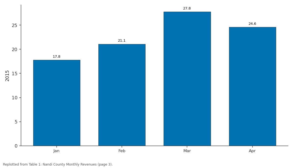
2015: Jan vs Feb vs Mar vs Apr
Replotted from Table 1 (page 3) of the original paper. Every bar is the paper's own table value.
View source evidence ↗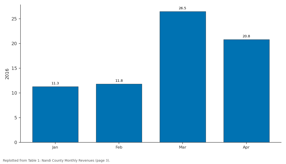
2016: Jan vs Feb vs Mar vs Apr
Replotted from Table 1 (page 3) of the original paper. Every bar is the paper's own table value.
View source evidence ↗Figures & tables
From the original paper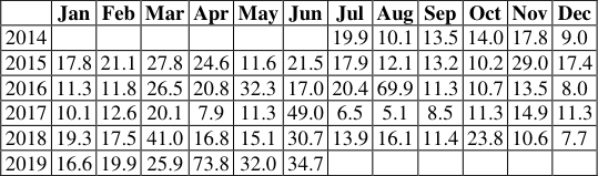 Table 1
 Table 2
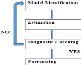 Figure 1
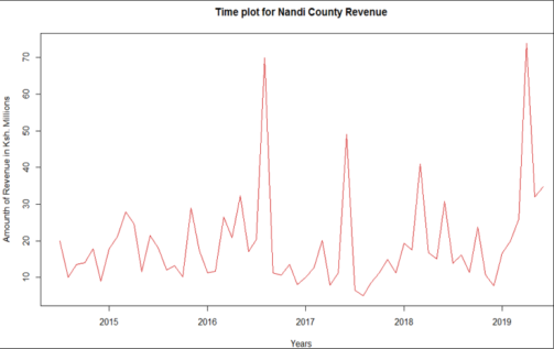 Figure 2
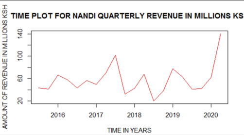 Figure 3
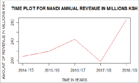 Figure 4
 Table 3
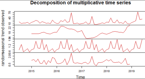 Figure 5
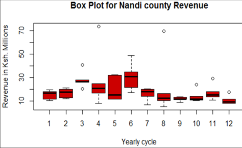 Figure 6
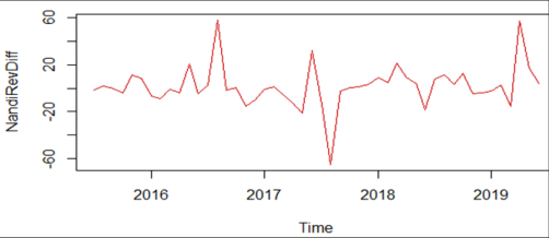 Figure 7
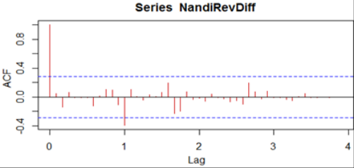 Figure 8
 Table 7
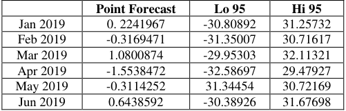 Table 8
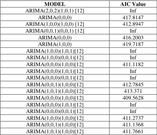 Table 4
 Table 1
 Table 5
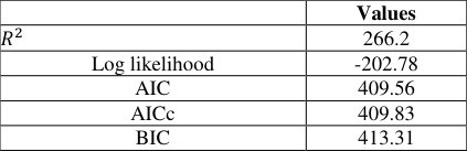 Table 6
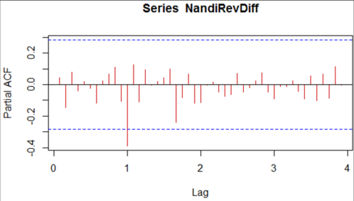 Figure 9
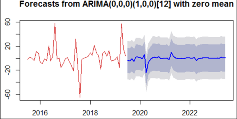 Figure 10
 Table 10
Introduction
The constitution of Kenya requires that the NG allocates the CGs a minimum of fifteen percent (15%) of the income from the last audited books of accounts. The amount allocated alone is not enough for CGs to finance their budgets and thus the need for OSR. The CG of Nandi has been raising its OSR through a number of sources referred to as Revenue Streams. They include business permits, liqour licensing, plot rents, land rates, house and stall rents, parking fees, market fees, cess, slaughter fees. The revenues are collected daily, monthly and annually. This study analyzed the CG of Nandi OSR from 2014/15 to 2019/2019 FY and forecasted the amounts to be collected in fours to come.
Statement of the Problem
County Government of Nandi has been using simple descriptive statistical techniques such as charts, bar, and line graphs to represent data on revenue collections. The techniques highlighted above have not been able to inform the CG of the seasonal trends associated with the collection of revenues over the years, neither does it inform on the amount of revenues likely to be collected in the future. This study, therefore, used a time series model known as Seasonal Autoregressive Integrated Moving Average (SARIMA) model to analyze the County Government of Nandi revenue, came up with a model that projected the amount of revenues to be collected in the future. This eliminates the problem of planning for the unknown and an unpredictable future.
Objectives of the Study 1.3.1 General Objective
To Perform Time Series Analysis of Nandi County Government Revenue Using Seasonal Autoregressive Integrated Moving Average (SARIMA) Model.
Specific Objectives
1. To analyze patterns of Nandi County revenue for the period 2014/15 to 2018/19 FY. 2. To fit a SARIMA model for the Nandi county revenue data for the period 2014/15 to 2018/19 FY 3. To forecast, using the fitted model, Nandi county revenue to be collected in the next four years.
Limitations of the study
1. COVID-19 pandemic to some extent interfered with the study forecast timetable more significantly the 2 nd and 3 rd quarters of 2020. 2. Time factor in putting multiple pieces of information per revenue stream together with the aim of forecasting revenues per stream. [1] used a SARIMA model to analyze tomato prices at wholesale level in Turkey. Tomato prices for the period from 2000 to 2010 were analyzed. The results obtained from this study showed that the prices of tomatoes in Turkey did not show any trend towards an increase or a decrease, in other words, the prices exhibited a stationary structure. The forecasts predicted from the SARIMA (1,0,0) (1,1,1)12 model which was chosen to determine the course of the prices of the next 3 years showed that any significant changes would not occur in Real Tomato Prices by the end of 2014.
Literature Review
Literature Review
Research Methodology 3.1 Data Source
This study used the secondary data obtained from the CG of Nandi, Revenue department. The data majorly comprised the amounts of revenue collected monthly from 2014/15 to 2018/19 FY.
Method of Analysis
Time series analysis was used to model the CG of Nandi revenue collected for a period of four years and forecasted the amount projected to be collected in four years to come. The general form of SARIMA as proposed by Box and Jenkins (1976) [3] and Kendall and Ord(1990) was used. Data were analyzed using R-Software. The ARIMA model is for non-seasonal non-stationary data.
Box and Jenkins have generalized this model to deal with seasonality. Their proposed model is known as the Seasonal ARIMA (SARIMA) model. In this model seasonal differencing of appropriate order is used to remove nonstationarity from the series. Each of the autoregressive and moving average processes has both the seasonal and nonseasonal parts. However, the distribution of the correlogram is the determining factor for the choice of the class of ARIMA or SARIMA model. The reason for the use of SARIMA (p, d, q)(P, D, Q)12 in this research work is that the revenue data were recorded on monthly basis. The seasonality period is 12.
The general form of seasonal model SARIMA(p, d, q) (P, D, Q)s is given by:
Where {𝑊 𝑡 } is the nonstationary time series, {𝑊 𝑡 } is the usual Gaussian white noise process. s is the period of the time series. The polynomials φ(B) and θ(B) of orders p and q represent the ordinary autoregressive and moving average components. The seasonal autoregressive and moving average components are Φ 𝑃 (𝐵 𝑆 ) and Θ 𝑄 (𝐵 𝑆 ), where 𝑃 and 𝑄 are their orders. ∇ d and ∇ 𝑆 𝐷 are ordinary and seasonal difference components. 𝐵 is the backshift operator. The expressions can be shown as follows;
This study focused on the amount of revenue collected monthly. The seasonal period of the series 𝑠 = 12. Equation (3.1) may therefore be written as:
The general forecasting equation is given by:
The mathematical formulation of a SARIMA (p,d,q)×(P,D,Q)s model in terms of lag polynomials is given below;
Here 𝑍 𝑡 is the seasonally differenced series.
Forecasting comprises four steps i.e Model Identification, Parameter estimation, diagnostic checking, and forecasting (Gujarati, 2004). This process is iterative in that it will have to be repeated until a desirable model of the data is identified.
Data Analysis, Presentation and Interpretation 4.1 Descriptive Data Analysis
The monthly revenue data in millions were presented as follows;
Table 1: The summary shows that the average amount of revenue that CG of Nandi collected per month is Ksh. 19.29 million. The least and the maximum amounts ever collected is Ksh. 5.10 million and Ksh. 73.80 million. The average amount collected quarterly was Ksh. 57.87 million. The least and the highest amount collected quarterly was Ksh. 20.10 million and 140.50 million respectively. Yearly, the average amount collected was Ksh. 231.4 million. The least and the maximum amount ever collected was Ksh. 197.9 and 286.3 million respectively.
| — | Jan | Feb | Mar | Apr | May | Jun | Jul | Aug | Sep | Oct | Nov | Dec |
|---|---|---|---|---|---|---|---|---|---|---|---|---|
| 2014 | 19.9 | 10.1 | 13.5 | 14.0 | 17.8 | 9.0 | ||||||
| 2015 | 17.8 | 21.1 | 27.8 | 24.6 | 11.6 | 21.5 | 17.9 | 12.1 | 13.2 | 10.2 | 29.0 | 17.4 |
| 2016 | 11.3 | 11.8 | 26.5 | 20.8 | 32.3 | 17.0 | 20.4 | 69.9 | 11.3 | 10.7 | 13.5 | 8.0 |
| 2017 | 10.1 | 12.6 | 20.1 | 7.9 | 11.3 | 49.0 | 6.5 | 5.1 | 8.5 | 11.3 | 14.9 | 11.3 |
| 2018 | 19.3 | 17.5 | 41.0 | 16.8 | 15.1 | 30.7 | 13.9 | 16.1 | 11.4 | 23.8 | 10.6 | 7.7 |
| 2019 | 16.6 | 19.9 | 25.9 | 73.8 | 32.0 | 34.7 |
Table text extracted from the original PDF; superscript letters are shown inline. The original table image is below.
View original table image
Time Plot for Nandi County Revenues
Time plot for monthly, quarterly, and yearly amounts of revenues collected is given as follows;
Decomposition of the Time Series
The monthly revenue time series were decomposed in an attempt to check the existence of a seasonal trend. The figure above shows how the monthly time series were decomposed into random, seasonal, and trend components.
The trend component shows the behavior of the revenues as they were collected, whether they were rising or declining. In this particular case, the revenues rose from 2014/15 FY to 2016/17 FY, declined in 2017/18 FY, and rose steadily thereafter. The random components represent all the components that did not fit in the trend and the seasonal part.
The seasonal components show the periodic behavior of the revenues within a yearly cycle. This confirms the significance of choosing the SARIMA model.
Box Plot
The Box-Plot was plotted to study the seasonal pattern for revenue collection in Nandi County. From July, the revenues decrease steadily to its worst in September, rises slightly in October and November, and drops again in December. This cycle repeats annually and may be used to predict the expected future seasonal pattern.
Test of Hypothesis
It was established whether the mean amounts of revenues collected were the same for all the months across the five years. 𝐻 0 : No difference in the mean amount of monthly revenue collected 𝐻 1 : There is a significant difference in the mean amount of monthly revenue collected. Since p-value <0.05, we, therefore, reject the null hypothesis.
There is a statistically significant difference in the mean amount of revenue collected per month. From the plots, the only significant autocorrelation is at lag 1, showing an MA (1) pattern. Also, partial autocorrelations are significant, showing an AR (1). Several models were suggested but auto.arima function was used to choose the best SARIMA model with respect to the least AIC value. The table below shows the various models which were identified before choosing the most suitable model. Inf ARIMA(0,0,0) 417.8147 ARIMA(1,0,0)(1,0,0) [12] 412.8947 ARIMA(0,0,1)(0,0,1) [12] Inf ARIMA(0,0,0) 416.2003 ARIMA(1,0,0) 419.7187 ARIMA(1,0,0)(1,0,1) [12] Inf ARIMA(1,0,0)(0,0,1) [12] Inf ARIMA(0,0,0)(1,0,0) [12] 411.1182 ARIMA(0,0,0)(1,0,1) [12] Inf ARIMA(0,0,0)(0,0,1) [12] Inf ARIMA(0,0,1)(1,0,0) [12] 412.7845 ARIMA(1,0,1)(1,0,0) [12] 413.371 ARIMA(0,0,0)(1,0,0) [12] 409.5628 ARIMA(0,0,0)(1,0,1) [12] Inf ARIMA(0,0,0)(0,0,1) [12] Inf ARIMA(1,0,0)(1,0,0) [12] 411.2737 ARIMA(0,0,1)(1,0,0) [12] 411.1368 ARIMA(1,0,1)(1,0,0) [12] 411.7661
Trend Differencing for the Amount of Monthly Revenue Collected
The best model was chosen as SARIMA (0,0,0)(1,0,0) [12] with zero mean. The model had the least AIC value of 409.56.
Parameter Estimation
After identification of the best model, it was evidenced that SARIMA (0,0,0)(1,0,0) [12] was the best model. The estimated parameters and model fits are shown below. 𝐻 0 : The SARIMA model is suitable for the data 𝐻 1 : The SARIMA model is unsuitable for the data.
The results were as follows;
Train and Test Method
The Train and Test method was also used to test the suitability of the model. A new model was fit while omitting the data for the last six months of the last financial year. The same model was used to forecast the amounts of revenues for the final. These projected amounts were then compared with the original data. The original data for the last six months is as follows; When the original data is compared with the projected data, there is a slight variance. The projected values move around the mean. The mean of the original and the forecasted data are 33.8 and 31.0 respectively. The variance of the projected data from the original data is -2.8 which is a small difference. This leads to the conclusion that the SARIMA model was suitable for the data.
Forecasting the Amounts of Revenues
The monthly amounts of Nandi County Government revenues were projected using the fitted model SARIMA(0,0,0)(1,0,0) [12]. The forecasts show the amounts of revenues collected by the Nandi County government will continue displaying the seasonality which was witnessed in the data. An overview of the forecasted amounts in millions are given in the table below; The average amounts of monthly forecasted revenues for the projected four years is Ksh. 34.97 million per month. The least forecasted amount is Ksh. 8.14 million and the highest possible amount is Ksh. 44.63 million.
Summary, Conclusions and Recommendations
The analysis showed that the Nandi county revenue department collects an average monthly revenue amounting to Ksh. 19.29 million. The revenues collected followed a yearly seasonal trend. The revenues increases from January to its peak in June. Then it declines steadily to its worst in September, rises slightly, and falls again in December. This is a cycle that revenues collected follow annually.
The SARIMA model SARIMA (0,0,0)(1,0,0)[12] used to forecast the Nandi County OSR proved to fit well in the data. This is attributed to the fact that the data (amounts of revenues collected monthly) follow a seasonal trend. The amounts forecasted also followed the same seasonal trend as the original data.
Figures and tables from the paper
| — | Min. | 1st Qu. | Median | Mean | 3rd Qu. | Max. |
|---|---|---|---|---|---|---|
| Monthly | 5.10 | 11.30 | 16.35 | 19.29 | 21.20 | 73.80 |
| Quarterly | 20.10 | 41.92 | 53.10 | 57.87 | 67.08 | 140.50 |
| Annual | 197.9 | 208.7 | 219.5 | 231.4 | 244.7 | 286.3 |
Table text extracted from the original PDF; superscript letters are shown inline. The original table image is below.
View original table image
| — | Point Forecast | Lo 95 | Hi 95 |
|---|---|---|---|
| Jan 2019 | 0. 2241967 | -30.80892 | 31.25732 |
| Feb 2019 | -0.3169471 | -31.35007 | 30.71617 |
| Mar 2019 | 1.0800874 | -29.95303 | 32.11321 |
| Apr 2019 | -1.5538472 | -32.58697 | 29.47927 |
| May 2019 | -0.3114252 | 31.34454 | 30.72169 |
| Jun 2019 | 0.6438592 | -30.38926 | 31.67698 |
Table text extracted from the original PDF; superscript letters are shown inline. The original table image is below.
View original table image
| MODEL | AIC Value |
|---|---|
| ARIMA(2,0,2)(1,0,1) [12] | Inf |
| ARIMA(0,0,0) | 417.8147 |
| ARIMA(1,0,0)(1,0,0) [12] | 412.8947 |
| ARIMA(0,0,1)(0,0,1) [12] | Inf |
| ARIMA(0,0,0) | 416.2003 |
| ARIMA(1,0,0) | 419.7187 |
| ARIMA(1,0,0)(1,0,1)[12] | Inf |
| ARIMA(1,0,0)(0,0,1)[12] | Inf |
| ARIMA(0,0,0)(1,0,0)[12] | 411.1182 |
| ARIMA(0,0,0)(1,0,1)[12] | Inf |
| ARIMA(0,0,0)(0,0,1)[12] | Inf |
| ARIMA(0,0,1)(1,0,0)[12] | 412.7845 |
| ARIMA(1,0,1)(1,0,0)[12] | 413.371 |
| ARIMA(0,0,0)(1,0,0)[12] | 409.5628 |
| ARIMA(0,0,0)(1,0,1)[12] | Inf |
| ARIMA(0,0,0)(0,0,1)[12] | Inf |
| ARIMA(1,0,0)(1,0,0)[12] | 411.2737 |
| ARIMA(0,0,1)(1,0,0)[12] | 411.1368 |
| ARIMA(1,0,1)(1,0,0)[12] | 411.7661 |
Table text extracted from the original PDF; superscript letters are shown inline. The original table image is below.
View original table image
| — | Values |
|---|---|
| 𝑅2 | 266.2 |
| Log likelihood | -202.78 |
| AIC | 409.56 |
| AICc | 409.83 |
| BIC | 413.31 |
Table text extracted from the original PDF; superscript letters are shown inline. The original table image is below.
View original table image
| Year | Forecasted revenues in ksh. Millions | — | — | — |
|---|---|---|---|---|
| April | June | September | December | |
| 2020 | 8.1425984953 | 30.3068260088 | 35.170534538 | 34.0337796868 |
| 2021 | 44.631832611 | 35.3629084364 | 34.899556799 | 35.3749396888 |
| 2022 | 30.942908439 | 34.8191073869 | 35.278158453 | 35.0793566701 |
| 2023 | 36.932800990 | 35.3118018324 | - | - |
Table text extracted from the original PDF; superscript letters are shown inline. The original table image is below.