
Research article · 2022 · Full text
International Journal of Statistics and Applied MathematicsNumerical integration of locally peaked bivariate functions
Volume 7(3) · Pages 43–48 · DOI: 10.22271/maths.2022.v7.i3a.823 ↗
Research areasMathematical functions and polynomialsMathematical Approximation and IntegrationScientific Research and Discoveries
Abstract
Author-writtenThe aim of this paper is to compare the relative accuracies between deterministic and stochastic methods for solving bounded integrals numerically to observe which methods tend to function well and converge to a small amount of error based on computational resources. For the deterministic method, the Gauss-Legendre quadrature method has been selected and for the stochastic method, the Monte Carlo integration has been selected. For each case, the number of variables will be adjusted to observe the effect on error.
Summary
Source-checkedPlain-language reading of the full paper, prepared with AI and checked against the text. Each point links to the authors' own words.
Why it matters
- Numerical integration is used to approximate the value of definite integrals when analytical methods are difficult or impossible to apply. View evidence ↗
- Numerical methods are advantageous when anti-derivatives are not elementary functions or when they offer savings in time and processing power compared to analytical solutions. View evidence ↗
- The 'curse of dimensionality' refers to the exponential growth of function evaluations required as the number of variables in an integral increases. View evidence ↗
The question
- The study aims to compare the relative accuracy and convergence of deterministic and stochastic numerical integration methods based on available computational resources. View evidence ↗
What they did
- The researchers selected the Gauss-Legendre quadrature as the deterministic method and Monte Carlo integration as the stochastic method. View evidence ↗
- Two bivariate functions were tested: an exponential function with a true integral value of 8.5574 and a trigonometric function with a true value of 3.9526. View evidence ↗
What they found
- For the first function using Monte Carlo integration, the error dropped from 29% at N=10 to nearly 0% at N=100. View evidence ↗
- Using Gauss-Legendre for the first function, the error started at 9% for k=2 and was reduced by 90% when nodes were increased to k=3. View evidence ↗
- For the second function using Gauss-Legendre, the error remained high, starting at -42.999% for k=2 and only decreasing to 10.941% by k=5. View evidence ↗
What it means
- The authors conclude that for stochastic methods, the error is inversely proportional to the number of samples. View evidence ↗
- The authors state that the Monte Carlo method is immune to the curse of dimensionality and is not resource intensive. View evidence ↗
- The authors suggest future experiments with logarithmic functions to test how the methods handle rapidly increasing areas under the graph. View evidence ↗
Visual summary
2 visualsIllustrations explain the paper; charts are replotted from the paper's own table values.
Comparison Framework
AI-generated conceptual illustration (A 3D mathematical surface plot of a bivariate function with a sharp, local peak). It explains the idea and does not show study data.
View source evidence ↗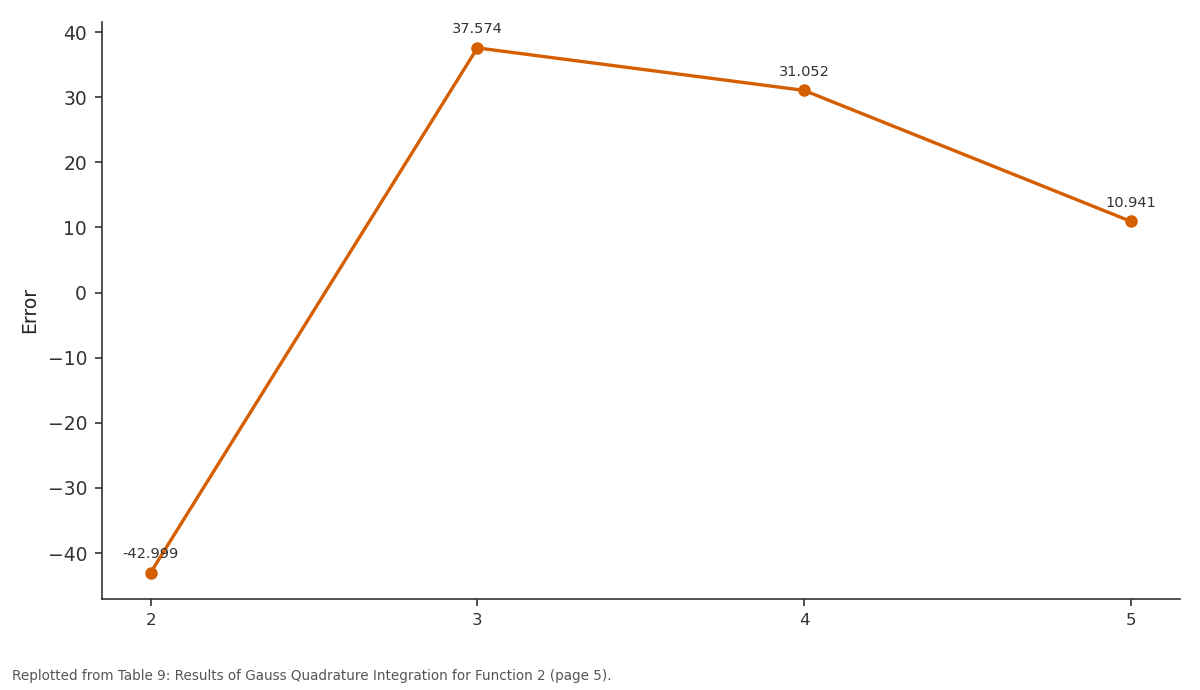
Error: 2 vs 3 vs 4 vs 5
Replotted from Table 9 (page 5) of the original paper. Every bar is the paper's own table value.
View source evidence ↗Figures & tables
From the original paper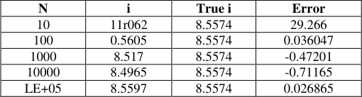 Table 1
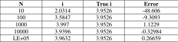 Table 2
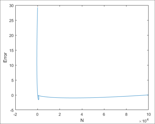 Figure 1
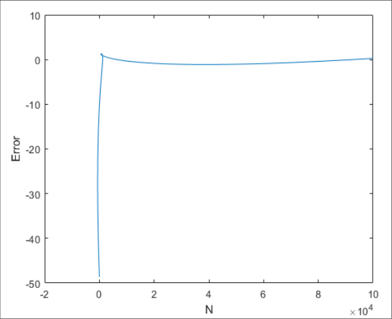 Figure 2
 Table 5
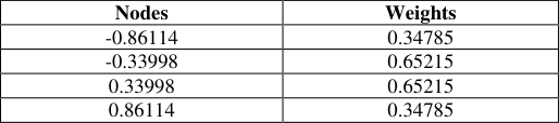 Table 6
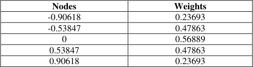 Table 7
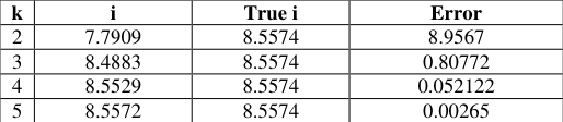 Table 8
 Table 3
 Table 4
 Table 9
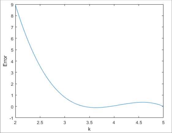 Figure 3
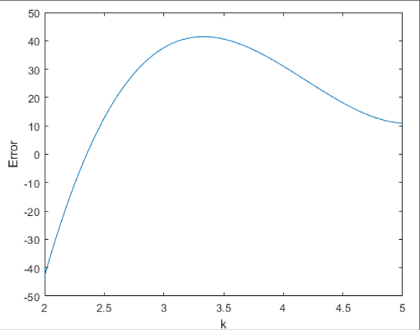 Figure 4
Introduction
Numerical integration is the process of the numerical approximation of the answer of a definite integral over a set of defined limits. Typically, most integrals can be solved using analytical methods such as integration by substitution, integration by parts and others. However, sometimes the integrals tend to become difficult or impossible to solve using typical analytical methods. Therefore, to find the integrals of such functions, we must rely on the numerical methods which are algorithms that aid in finding the numerical value of the definite integral of a function. The objective of our paper will be the numerical calculation of definite integrals in two variables. Of the algorithms used, there is a term known as numerical quadrature which is another term for numerical integration. Specifically, this term is used to represent one dimensional integrals, which are integrals in one variable. Other terminologies are also used which define higher dimension integrals as cubature [1] . Thus, numerical quadrature can be defined as the estimated answer to the following integral:
This is an integral of a function from a defined range, known as a definite integral, which often has varying degrees of accuracy. For this reason, there are two conditions that must be satisfied. Firstly, the function should be smooth over a small, limited amount of dimensions. Secondly, the function should be bounded. Provided that these two conditions are satisfied, we can come up with many different numerical methods to find estimates of the solution of the integral to a certain level of precision. There are also multiple advantages of numerical integration over analytical techniques. Firstly, the integrand may only be required at certain points, for example, through sampling, which is why many embedded applications tend to use numerical integration instead of analytical integration. Sometimes it's also possible where we know the technique for the analytical integration, but cannot find the anti-derivative which exists as an elementary function. Finally, sometimes, it's possible to calculate the analytical solution but it's easier to find the solution numerically which can save not only time but also processing power. The basic definition of any numerical integration algorithm can be defined as the combination of the integrands' evaluations which leads to an approximate solution to the integral. The integration points are finite in number and integrands are calculated at these points.
Then, by calculating the weighted sum of these values, we can approximate the integral. These integration points and weights vary from method to method and affect the level of accuracy of the calculation. One of the critical aspects of the analysis of numerical techniques is to assess the trend of the approximate error. The ideal method for this is to specify the error as a function of the number of numerical evaluations. Usually, the quality of the method is judged by assessing which function yields minimal error while keeping number of iterations minimum. These algorithms are then considered to be the better algorithms because they reduce the number of machine cycles by reducing the number of mathematical operations that have to be conducted. This eventually leads to a lower error. This is particularly considerable in cases where the time taken per iteration is high and the integrand to be evaluated is complex. There is a category of numerical integration which is classified as a brute-force numerical integration. This is only applicable to integrands which are piecewise and continuous in nature, and have bounds specified to them. This leads to a possibility of completing the integral using small increments in the values of the variables using the bounds of the function as limits. Most quadrature rules are usually designed to compute integrals in one variable only. There are techniques to extend these methods to multiple variables which involve the consideration of the multiple integral as a series of single one dimensional integrals using Fubini's theorem. This approach, however, causes the function evaluations to grow in an exponential nature as the number of variables increases. Consequently, this is known as the curse of dimensionality. Three techniques are known to overcome this problem. One of these techniques is known as the Monte Carlo integration. This technique uses random distributions to carry out numerical integration. This method computes numerically a definite integral over a given bound and is a subset of a series of methods known as Monte Carlo methods. This is an example of a stochastic method in which random points are chosen between the bound of the integrand at which this integrand is evaluated. Other methods compute the integrand at a regular grid [2] . The Monte Carlo method is quite useful for integrals of higher dimensions [3] . There are also multiple methods which can be used to carry out the Monte Carlo integration. Some examples of these methods are particle filter, mean-field particle filter, uniform sampling, etc. Two of the most common methods are finite element method and boundary element methods. These methods are quite popular in engineering applications. Some differential equations, considered to be boundary value problems, can be numerically solved using discretization which results in a series of linear algebraic equation which allows us to approximate a solution to the problem. The accuracy of these methods rely on the quadrature method used for the integration of the functions of the elements. A derivation of integral equations for solutions of different boundary value problems have been defined in [4] . There are other techniques of numerical integrations in one and multiple dimensions using Gauss quadrature methods [5] . For curves that are smooth, and exist over finite intervals often defined as [a, b], the interval can often be linearly converted to the standardized interval [-1,1] in which we can apply the easier method known as the Gauss Legendre quadrature. The Gaussian quadrature methods are a series of methods that can be classified as deterministic methods. The Gauss Legendre quadrature allows the numerical integration of a function to a certain degree of accuracy; however, the process leads to a slowly converging error for functions based on logarithms. In such cases, other weighted quadrature for Gaussian methods are recommended. The Gauss Legendre quadrature allows the numerical integration of a function to a certain degree of accuracy; however, the process leads to a slowly converging error for functions based on logarithms. In such cases, other weighted quadrature for Gaussian methods is recommended.
Methodology Equations to Be Integrated
For the purposes of our paper, we will simulate the numerical integration of two functions by using two separate methods. The first method will be a stochastic method, which will be the Monte Carlo method. The second method will be a deterministic method, or a quadrature method. In each case, the limits for the integration will be taken as [-1,1].
1) First Equation
The first equation to be integrated will be
This can be analytically integrated to give us the result:
Hence, the true value of this integral is 8.5574.
2) Second Equation
The second function to be integrated will be
This can be analytically integrated to give us the result:
Hence, the true value of this integral is 3.9526.
A) Monte Carlo Integration
The first method of integration that we will implement will be the Monte Carlo integration. This is a stochastic form of integration which relies on random numbers. Since the integral of a function is equivalent to the area under the graph of the function plotted, we can use this method to estimate the integral of the function. The method consists of starting with the goal of finding the integral of a function over a given range. For our experiment, our range is going to be limited to [-1,1]. Therefore, we have to find the area of the function between -1 and 1. To do this, we can take a random value of x between -1 and 1 and multiply the value of the function with this given value of x to find the area of the rectangle. This is an approximation of the integral of a function. The Monte Carlo method approximates the integral value by taking the average of the area of the rectangles which is computed for a random value of x between the given range, in this case, -1 and 1. As we keep adding the area of the rectangles and then find the average value of the sum, we can approximate our answer with more and more accuracy. One of the consequences of this is that, the over-estimated areas are compensated for by the under-estimated areas. This leads us to the derivation for the Monte Carlo method:
And Ω is a subset of R m where all the values of x,
And N is the number of uniform samples. These points are sampled and this technique relies on the law of large numbers that states:
Using the equation 5, we can estimate a value for the integral which will be done for both the given functions.
For our experiment, we varied the values of N to observe the effect of increasing the sample size on the accuracy of the algorithm to confirm that the error is inversely related to the sample size. Furthermore, we solve equation 6 to find the value of V which comes out to be 4.
B) Gauss-Legendre Quadrature Integration
In Numerical Analysis, a classification of algorithm for the approximation of the area under the curve of a function is the quadrature rule. This technique consists of taking the weight sum of the function values at predefined points between the given range of the function. There is a sub-classification of these rules known as the Gaussian quadrature rules wherein the rule yields an exact result for polynomials of degrees up to 2n-1 with weights w i for i=1,…,n which is then known as the n-point Gaussian Legendre Quadrature rule. This method requires the domain of the function to be [-1, 1] which allows this rule to be defined as:
And this method has been known to be exact for polynomials of degree 2n-1 or less. This rule is specifically known as the Gauss-Legendre quadrature rule. There are other limitations to the use of this algorithm. For example, this rule is most accurate when the domain is [-1,1] and the integrand can be written as:
where a and b are both greater than -1 and g(x) is a low degree polynomial.
Furthermore, the Gauss-Legendre quadrature requires the weights of the function to be known which can be calculated using the equation:
For the interval [-1,1], the quadrature rules can be calculated a varying number of points. For the purposes of our experiment, we varied the number of points from 2 to 5; this is due to the fact that selecting one point leads to an undefined value of the integral [6] .
In the case of the limits being something other than [-1, 1], such as [a, b], we can conduct a coordinate transform to change the coordinates into [-1,1] using the following equation:
Consequently, for the second variable, the co-ordinate transform becomes:
Furthermore, to conduct a Gauss-Legendre for a bivariate function, we have to extend the one-dimensional formula to a two-dimensional formula. Conversion of the one-dimensional formula into a twodimensional formula is relatively simple. We have to simple perform repeated integrations as per the number of variables to achieve the two dimensional formula.
Thus, from equation 9, we can derive:
Analysis
For the purposes of our experiment, we have compared the relative accuracies of one stochastic method and one deterministic method. Due to the different nature of the two types of numerical integration methods, it's difficult to compare their performances with each other. However, we can study the effects of adjusting different parameters within the methods themselves to observe their accuracy.
A) Monte Carlo Integration
For stochastic methods such as the Monte Carlo integration method, the variable that can be adjusted is the number of samples. Consequently, we adjusted the number of samples from 10 1 to 10 5 and observed the effect of the number of samples to the error present. From the implementation of the Monte Carlo integration for function 1, we observe a relatively large error of 29% for a small sample size of N = 10. However, as we increase it to a sample size of N = 100, the error is significantly reduced to nearly 0%). Increasing the sample size further leads to smaller amounts of reduction in errors, as well as a small fluctuation in the error. Consequently, we may want to stop the sample size at 10 2 if our target error margin is below 1% or at N = 10 5 if smaller errors of less than 0.02% are required. Another trend in the error that we can observe is the oscillating nature of the error from positive to negative. This can be further studied by observing continuous increments of the number of sample size; however, such a test is resource intensive and the results would be difficult to show. From the figure above, we can observe that the trend of the error approaches zero as the number of samples increases. The plot would be smoother if the number of samples were reduced to observe the trend of errors for a lower number of samples; the sharp turn in the graph is a result of the large number of samples compared to the small error size. The table above displays the results of the implementation of the Monte Carlo integration for function 2. As observed, with a small sample size of N = 10, the error is quite large; 48%, as in the previous case. The increase to N = 100 reduces this error to approximately 9% and N = 100 leads to a small error of 1%. Similar to the previous observation, the error reduces to below 1% at a sample size of N = 10 4 and small amounts of acceptable error of 1% can be obtained at N = 1000. The plot above shows a similar trend to the previous graph where as the number of samples increases, the error reduces to nearly zero. There is once again a sharp turn on the graph due to the large number of samples present compared to the small error.
B) Gauss-Legendre Quadrature
For deterministic methods such as the Gauss Quadrature methods, there are no longer a large number of random samples that are randomly selected. For the purposes of weighted Gauss Quadrature methods, we can compare the different values of weights or the number of selected points between the bounds which lead to the different values of weights. For our case, we selected the Gauss-Legendre Quadrature method which allowed us to compare the error with respect to the number of points.
Before proceeding with the Gauss-Legendre quadrature, it's important to use Equation 11 to calculate the weights of the npoint quadrature formula. To display the individual values, we specifically calculated the weights for different values of n. The results of this simulation are shown below: The results of the first execution of the simulation of the Gauss-Legendre integration lead to the conclusion that for function 1, the iterations proceed to start with a large error of 9% at k=2 which is then reduced by 90% when the number of nodes is increased to 3. The error shows a sharp decrease as the number of nodes is further increased. By fitting a polynomial to the trend of the error, we can observe the rapid descent towards the y-axis, showing that as the number of nodes k is increased, the error tends to approach zero. For more diverging functions, we can increase the number of nodes to trade processing power for higher accuracy. For the final part of our simulation, we can observe the trend of the error to be decreasing with a slight oscillation in the Gauss-Legendre integration. As we increase the number of points 'k' the error can visibly be seen to be decreasing. Consequently, we can expect the error to decrease further as the number of points increase and the number of weights increase. Once again, with more resources we can increase the number of points and observe the effect further to confirm this theory. The figure above displays the plot of the trend of the error versus the number of points 'k' which shows an initial large error that seems to oscillate a little and is expected to flatten out. We do expect the error to go further down towards zero provided that we increase the number of points 'k' which will eventually lead to an increase in the number of computational resources required.
Conclusion
To conclude our experimentation, we can observe that for stochastic methods that rely on a random number chosen from a large sample size, the error can be seen to be inversely proportional to the number of samples.
𝑒𝑟𝑟𝑜𝑟 ∝ 1 𝑁
And to be specific, this observation is quite similar to the true relationship between the error and the number of samples which, to be specific, is actually:
This seems to be the true observation for both of our experiments, for function 1 and function 2. Consequently, we can further experiment with different functions to observe the results for a logarithmic function to see how the method can keep up with the rapidly increasing area under the graph. This method also is not resource intensive on its own which reinforces the idea that the Monte Carlo method is immune to the curse of dimensionality. Secondly, for the deterministic methods such as weighted quadrature methods, we also observe that these methods also tend to overcome the curse of dimensionality by using weights that depend on the number of points chosen between two bounded limits given. This leads to the increasing accuracy of the system without leading too much into complex calculations. Consequently, we can observe the fact that the percentage error is inversely related to the number of points selected 'k'.
Figures and tables from the paper
| N | i | True i | Error |
|---|---|---|---|
| 10 | 11r062 | 8.5574 | 29.266 |
| 100 | 0.5605 | 8.5574 | 0.036047 |
| 1000 | 8.517 | 8.5574 | -0.47201 |
| 10000 | 8.4965 | 8.5574 | -0.71165 |
| LE+05 | 8.5597 | 8.5574 | 0.026865 |
Table text extracted from the original PDF; superscript letters are shown inline. The original table image is below.
View original table image
| N | i | True i | Error |
|---|---|---|---|
| 10 | 2.0314 | 3.9526 | -48.606 |
| 100 | 3.5847 | 3.9526 | -9.3093 |
| 1000 | 3.997 | 3.9526 | 1.1229 |
| 10000 | 3.9396 | 3.9526 | -0.32984 |
| LE+05 | 3.9632 | 3.9526 | 0.26659 |
Table text extracted from the original PDF; superscript letters are shown inline. The original table image is below.
View original table image
| Nodes | Weights |
|---|---|
| -0.7746 | 0.55556 |
| 0 | 0.88889 |
| 0.7746 | 0.55556 |
Table text extracted from the original PDF; superscript letters are shown inline. The original table image is below.
View original table image
| Nodes | Weights |
|---|---|
| -0.86114 | 0.34785 |
| -0.33998 | 0.65215 |
| 0.33998 | 0.65215 |
| 0.86114 | 0.34785 |
Table text extracted from the original PDF; superscript letters are shown inline. The original table image is below.
View original table image
| Nodes | Weights |
|---|---|
| -0.90618 | 0.23693 |
| -0.53847 | 0.47863 |
| 0 | 0.56889 |
| 0.53847 | 0.47863 |
| 0.90618 | 0.23693 |
Table text extracted from the original PDF; superscript letters are shown inline. The original table image is below.
View original table image
| k | i | True i | Error |
|---|---|---|---|
| 2 | 7.7909 | 8.5574 | 8.9567 |
| 3 | 8.4883 | 8.5574 | 0.80772 |
| 4 | 8.5529 | 8.5574 | 0.052122 |
| 5 | 8.5572 | 8.5574 | 0.00265 |
Table text extracted from the original PDF; superscript letters are shown inline. The original table image is below.
View original table image
| Nodes | Weights |
|---|---|
| -0.57735 | 1 |
| 0.57735 | 1 |
Table text extracted from the original PDF; superscript letters are shown inline. The original table image is below.
View original table image
| k | i | True i | Error |
|---|---|---|---|
| 2 | 5.652 | 3.9526 | -42.999 |
| 3 | 2.4674 | 3.9526 | 37.574 |
| 4 | 2.7252 | 3.9526 | 31.052 |
| 5 | 3.5201 | 3.9526 | 10.941 |
Table text extracted from the original PDF; superscript letters are shown inline. The original table image is below.
View original table image
References
4 in the original paper- Milovanović GV, Igić TS, Turnić D. Generalized quadrature rules of Gaussian type for numerical evaluation of singular integrals, undefined. Apr. 2015;278:306-325. Doi: 10.1016/J.CAM.2014.10.009.
- Numerical Recipes 3 rd Edition: The Art of Scientific Computing | Request PDF. https://www.researchgate.net/publication/234831331_Nu merical_Recipes_3rd_Edition_The_Art_of_Scientific_Co mputing (accessed Jan. 30, 2022).
- Newman WI, Rand RH, Newman AL. Dynamics of a nonlinear parametrically excited partial differential equation. Undefined. 1999;9(1):242-253. Doi: 10.1063/1.166397.
- Sladek V, Sladek J, Sator L. Meshless implementations of local integral equations for bending of thin plates, WIT Trans. Modelling Simul. 2012;53(XXXIV):15-26. Doi: 10.2495/BE120021.