
Research article · 2022 · Full text
International Journal of Statistics and Applied MathematicsThe Laplace transform decomposition method applied to the numerical solution of the food chain ecoepidemic model
Volume 7(1) · Pages 132–145 · DOI: 10.22271/maths.2022.v7.i1b.784 ↗
Research areasCOVID-19 epidemiological studies
Abstract
Author-writtenThe aim of this study is to theoretically investigate the model parameters of the food chain ecoepidemic model using the Laplace transform decomposition method. The first order autonomous differential equations governing the model were reduced via the Laplace transform and Adomian decomposition to an algebraic equation, where the inverse Laplace transform gives the pertinent parameters. The analytically obtained solution which is the partial sum of the infinite series is then treated with Pade approximation to improve its convergence. To validate the results obtained, we compare the numerical solution via LADM with other semi-analytical methods viz LADM-Pade and Daftardar-Jafari (DJM. The results obtained are presented in tables and figures. The comparison showed, there is excellent agreement between the methods. It is observed the method is valid, efficient, applicable, robust, and computationally convenient to handle both linear and nonlinear differential as well partial differential equations.
Summary
Source-checkedPlain-language reading of the full paper, prepared with AI and checked against the text. Each point links to the authors' own words.
Why it matters
- Trophic levels within food chains are essential components of ecology and biological sciences. View evidence ↗
- Mathematical modeling of food chains has increased in academic interest because of the critical role food plays in ecosystems. View evidence ↗
- Modern research in this area includes the study of diseases affecting various levels of predator-prey interactions and the role of parasites. View evidence ↗
The question
- The study aims to theoretically investigate the parameters of a food chain ecoepidemic model using the Laplace transform decomposition method (LADM). View evidence ↗
What they did
- The model consists of three trophic levels: top predators, intermediate predators, and a bottom prey population divided into infected and susceptible subpopulations. View evidence ↗
- The researchers used the Laplace transform and Adomian decomposition to reduce first-order autonomous differential equations to algebraic equations to find model parameters. View evidence ↗
- Pade approximation was applied to the partial sum of the infinite series solution to enhance its convergence. View evidence ↗
- The LADM numerical solutions were validated by comparing them with LADM-Pade and the Daftardar-Jafari method (DJM). View evidence ↗
What they found
- The comparison between LADM, LADM-Pade, and DJM showed excellent agreement in the results. View evidence ↗
- For top predators (W), the LADM and DJM methods yielded identical values of 1.00000 at t=0 and 0.80400 at t=0.2. View evidence ↗
- For intermediate predators (V), LADM and DJM both produced a value of 1.55500 at t=0.2. View evidence ↗
- For infected prey (I), LADM and DJM results were identical at t=0 (1.00000), t=0.2 (2.10000), and t=0.4 (1.60000). View evidence ↗
- For susceptible prey (S), LADM and DJM produced identical values of 0.00000 at t=0 and -1.84480 at t=0.2. View evidence ↗
What it means
- The authors conclude that the LADM is a valid, efficient, robust, and computationally convenient method for solving linear and nonlinear differential equations. View evidence ↗
- The final analysis indicates that the method is correct and efficient, requiring less computational effort. View evidence ↗
Visual summary
3 visualsIllustrations explain the paper; charts are replotted from the paper's own table values.
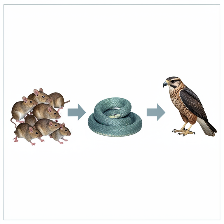
Food Chain Ecoepidemic Structure
AI-generated conceptual illustration (a three-level food chain consisting of a hawk, a snake, and a group of mice). It explains the idea and does not show study data.
View source evidence ↗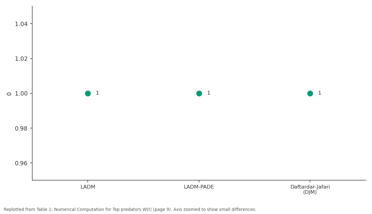
0: LADM vs LADM-PADE vs Daftardar-Jafari (DJM)
Replotted from Table 1 (page 9) of the original paper. Every bar is the paper's own table value.
View source evidence ↗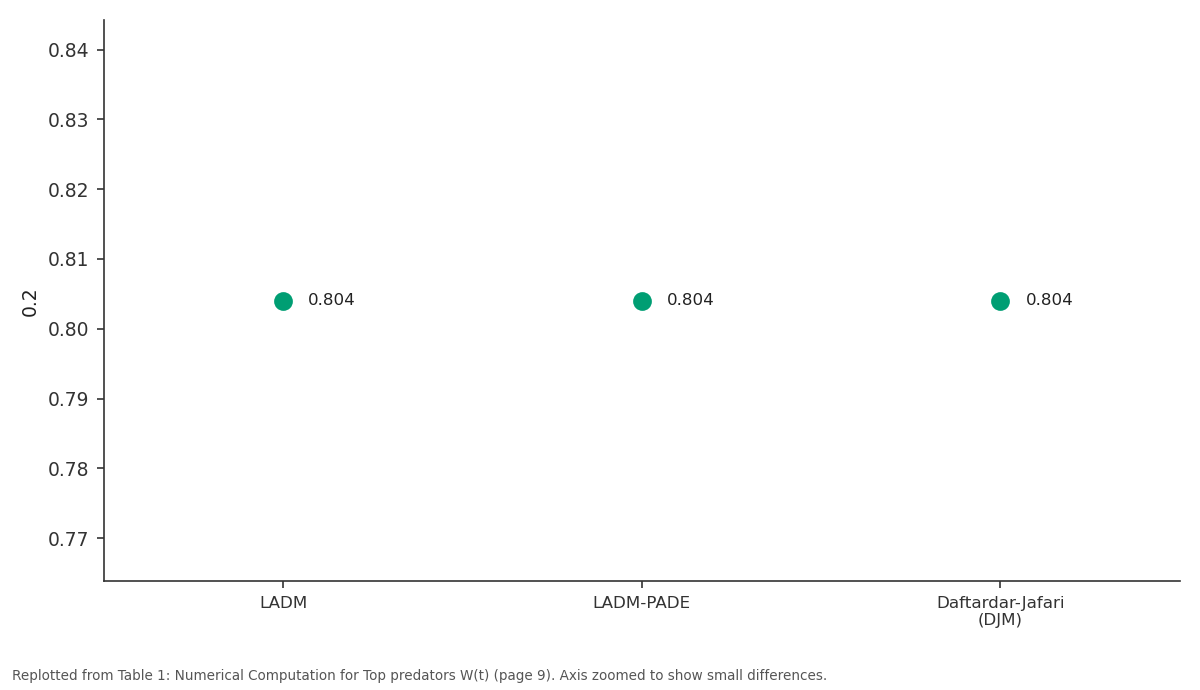
0.2: LADM vs LADM-PADE vs Daftardar-Jafari (DJM)
Replotted from Table 1 (page 9) of the original paper. Every bar is the paper's own table value.
View source evidence ↗Figures & tables
From the original paper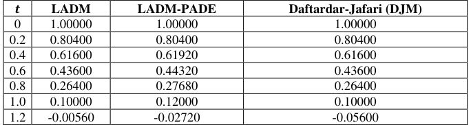 Table 1
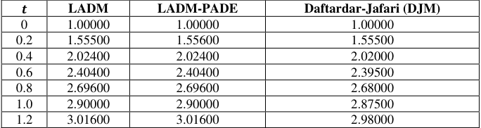 Table 2
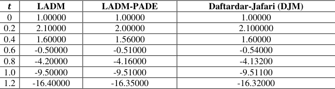 Table 3
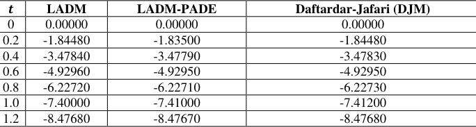 Table 4
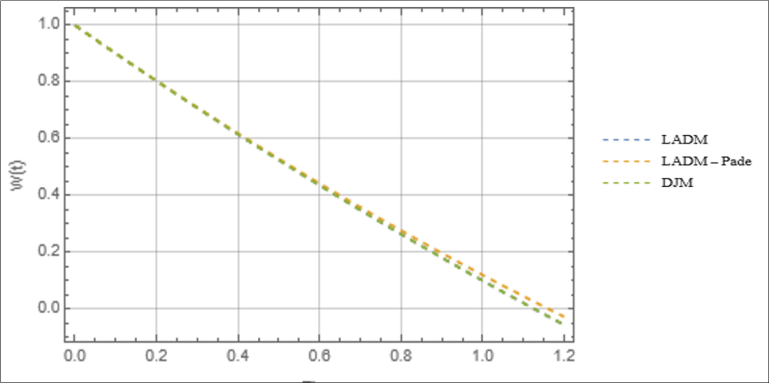 Figure 1
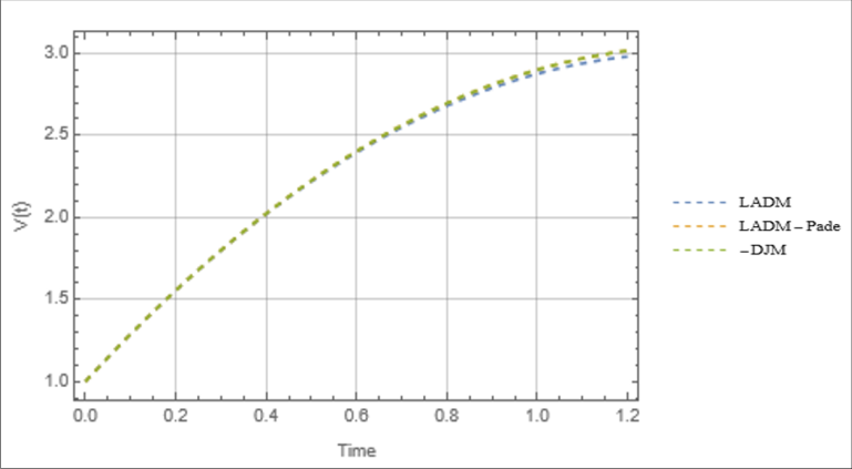 Figure 2
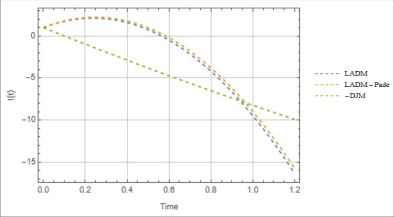 Figure 3
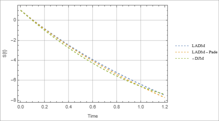 Figure 4
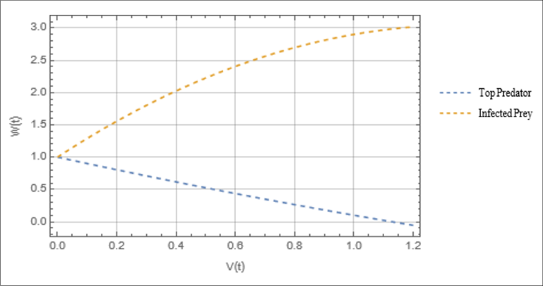 Figure 5
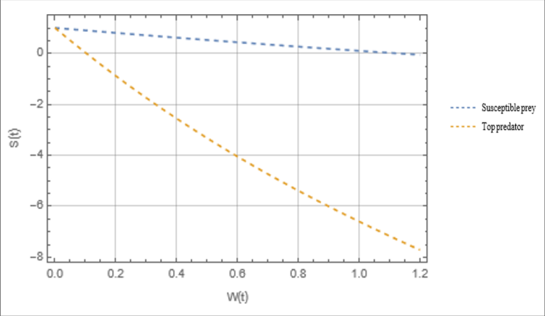 Figure 6
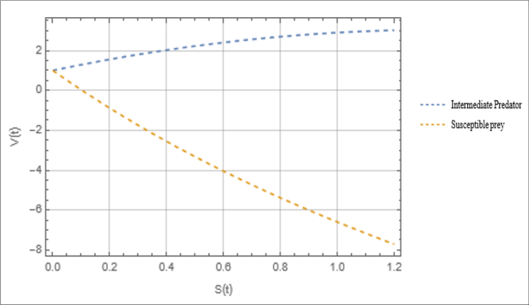 Figure 7
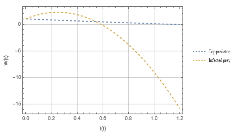 Figure 8
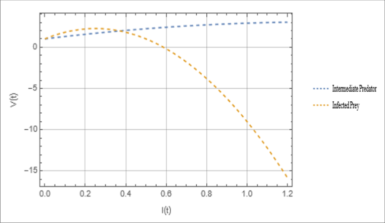 Figure 9
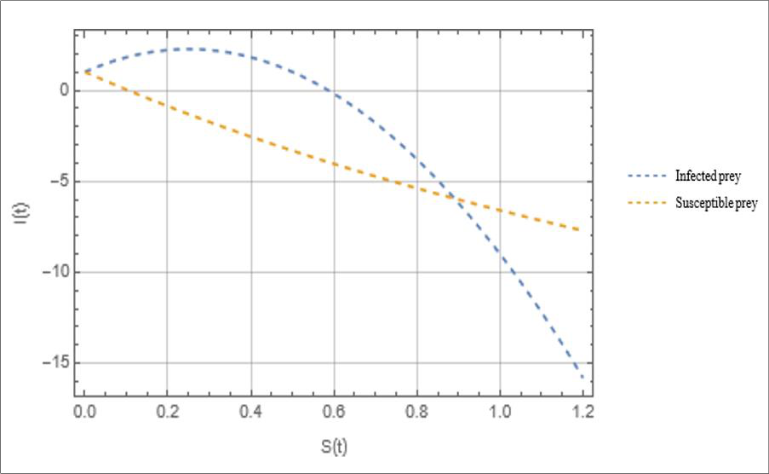 Figure 10
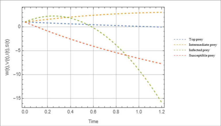 Figure 11
Introduction
In the field of ecology and biological sciences, trophic levels containing food chains play a pivotal role. Though this area of research is relatively nascent, researchers have done extensive research on this area with a view to understanding the ever-changing behaviour of the food web, modelling and analysing the changes in the pertinent parameters of the model. Earlier studies in the food chain model were carried out by Gard et al. 1979 [1] , Hallam and Gard 1980 [2] , Shukla 1981 et al. [3] and Kirlinger 1988 [4] . These studies were incisive and elaborate but couldn't incorporate all the intriguing factors that affects the food web and its attendant competition The extinction of the food web was modelled by [5] using a single variable parameter. The study of these mathematical models has grown among academics the world over especially in recent times due to the importance of food in the ecosystem. This now encompasses studies of diseases affecting the predator-prey both at the top and bottom, disease affecting interacting species in each population, effect of disease in aquatic lives, disease in parasitic and symbiotic environment and roles of parasites in ecology and many more. The dynamics and nature of diseases causing organism as well as others factor which breeds competition has equally been giving devoted attention by scholars. Most recently, Tripathi et al. 2004 [6] examined the prey-predator model with an emphasis on a reserved area. The study reveals that, when the parameter bearing the reserved area reaches a certain threshold, Hopf bifurcation sets in. It was further shown that better stabilizing influence results when predator refuse is introduced using Beddington-De Angeles functional response. This, the study opined is useful to national parks where prey and predators co-exist together, and the prey wished to be protected [7] . The Lokta-Volterra system with pest was investigated by Venturino 1993 [8] . In this study, the introduction of the pest was a check to keep predators at bay so the prey population wouldn't be utterly harmed by the predators [9][10] . independently analysed the prey-predator models including the SIS, SIR with infected prey. It was observed in this study that, when the prey population is vulnerable due to the disease introduced, the predators will persistently be present when indeed they are supposed to go extinction. Though most of these models are first order nonlinear autonomous differential equations, several approaches have been adopted to solve them for analytical and approximates solutions. These includes variational iteration method (VIM) [12][13] , Energy balance method [14][15] , Homotopy Analysis method (HAM) [16][17] , Homotopy perturbation method (HPM) [18] , Adomian decomposition method (ADM) [19] , Perturbation method [20] and others. Similarly, the modified Laplace Adomian decomposition method (LADM) have proved to be potent and extensively applied to solve several linear and nonlinear problems in contemporary times since it accelerates the rate of convergence of the approximate solution to the exact solution [21] . investigated the SIR model that incorporate child disease with preventive vaccine strategy using LADM. The system of linear and nonlinear PDEs have been studied by [22] . The study showed when more terms are taken, the convergence of the approximate solution was improved compared to ADM. The Duffing equation, Falkner-Skan equation, systems of nonlinear differential equations, nonlinear coupled PDEs, HIV infection model of CD4+Tcells, Newell-Whitehead-Segel equation, Systems of ordinary differential equations, linear and nonlinear Volterra Integral equation, Nonlinear Volterra Integro-differential equation, nth order integro-differential equation, two-dimensional viscous fluid with shrinking sheet, convection diffusion-dissipation equation, crime deterrence model, dynamics of atmospheric carbon dioxide have all been investigated using LADM [23][24][25][26][27][28][29][30][31][32][33] . Equally, the Daftardar-Jafari method (DJM) presented by Daftardar-Gejji Varsha, and Hossein Jafari have also been used to solve linear and nonlinear problems including PDEs, Jeffery-Hamel flow problems, nonlinear functional equation, fractional physical differential equation and fractional gas dynamics equation with coupled Burger's equation [34][35][36][37][38] . In this present research, we theoretically investigate the model parameters in the Ecoepidemic model of food chain consisting of three trophic levels namely: top predators, intermediate predators and a bottom subpopulation comprising infected and susceptible preys. The study is organized as follows. In section 1, the detailed introduction of the study is given. The basics of the Laplace Adomian decomposition method (LADM) is presented in section 2. The fundamentals of the Daftardar-Jafari method (DJM) are discussed in section 3. Section 4 gives the application of the LADM to the model to ascertain the model parameters. In section 5, the results are presented in tables, figures, and their explanation. Finally, the conclusion of the study is drawn in section 6.
Laplace Decomposition method (LADM)
In this subsection, we outline the basics of the fundamentals of the fusion Laplace transformation and Adomian decomposition method (LADM) Consider a functional differential equation of the form
Subject to the initial condition
Rearranging the above, we obtain the following relation for
Applying Laplace transform on both sides of Eq. ( 1), supposing the highest differential operator is of order two and using the differentiation property, we get
Next, we apply the inverse transform on both sides of Eq. ( 4), we obtain
Where 𝜙(𝑥) is the term arising from the first three terms on the right-hand side of Eq. ( 5) Next, we assume the solution as decomposing series in the form
Similarly, the nonlinear terms are written in terms of the Adomian polynomials
Where the 𝐴 𝑛 ′𝑠 represents the Adomian polynomials defined in the form
Plugging Eqs ( 6) and ( 7) into Eq. ( 5), we obtain
Matching both sides of Eq. ( 9), we obtain an iterative algorithm in the form
Then the solution of the differential equation is obtained as the sum of decomposed series in the form
Padé Approximation
In Mathematics and other applied sciences, power series representation of a function is usually in truncated form. To approximate these functions to an appreciable degree, polynomials are used because their singularities are easily noticeable in each finite region. However, the radius of convergence may not be large enough to contain two boundaries, for this reason, power series is not always the best method to approximate a function. To overcome this inherent hurdle, a new approximation is applied to the solution obtained using power series as a quotient of two functions with varying degrees in a finite interval. Pade approximation has been widely used to approximate several problems and has tremendous applications especially in computer calculation because it gives a better approximation without truncating its power series and still in problems where the series diverges. The different Pade approximants are obtained with the use of symbolic software Mathematica. [See 39 -42] A rational approximation to a function 𝑓(𝑥) on [𝑎, 𝑏] is the quotient of two polynomials, 𝑃 𝑁 (𝑥) and 𝑄 𝑀 (𝑥) of degrees 𝑁 and 𝑀 respectively. It is denoted by
Now consider the formal power series
Multiply both sides of Eq. ( 14) by a constant keep it unchanged, hence we impose the normalization condition.
Next, we require that 𝑃 𝑁 (𝑥) and 𝑄 𝑀 (𝑥) have non-common factors, so we write the coefficients of the 𝑃 𝑁 (𝑥) and 𝑄 𝑀 (𝑥) as follows
Using Eqs. ( 15) and ( 16), we multiply Eq. ( 13) by 𝑄 𝑀 (𝑥). This linearizes the coefficient equation. Its is given in detailed form as
Equating the coefficients of 𝑥 𝑁+1 , 𝑥 𝑁+2 , … , 𝑥 𝑁+𝑀 successively to zero, we obtain the system of Equations
For 𝑗 < 0, we define 𝑐 𝑘 = 0 for consistency. Setting 𝑏 0 = 1, Eq. ( 12) become a set of 𝑀 linear equations for 𝑀 unknown coefficients in the denominator.
Solving the above system in Eq. ( 18), the coefficients 𝑏 𝑖 for 𝑖 = 1,2, … . 𝑀 may be found. Since the coefficients of the numerator, 𝑐 0 , 𝑐 1 , 𝑐 2 , … . , 𝑐 𝑘 is known. We equate the coefficients of 1, 𝑥, 𝑥 2 , … , 𝑥 𝑁 , 𝑥 𝑁+𝑀 to obtain the remaining coefficients 𝑎 0 , 𝑎 1 , 𝑎 2 , … , 𝑎 𝑁 𝑥 0 : 𝑐 0 -𝑎 0 = 0
𝑥 𝑁 : 𝑐 0 𝑏 𝑁 + 𝑐 1 𝑏 𝑁-1 + 𝑐 𝑁 -𝑎 𝑁 = 0
Writing the above in explicit form, we obtain
In view of Eqs. ( 18) and ( 19), the numerator and denominator of the Pade approximant are all determined which agrees with the original series to the order of 𝑥 𝑁+𝑀. Now, to solve the system (19) for the set of unknowns, we assume that the Eqs. ( 18) and ( 19) are non-singular, so we can obtain the solution via the determinant.
To obtain the diagonal Pade approximants of different orders such as
⁄ ], we use symbolic software Mathematica
Application of LADM to the Epidemic Model
We consider the eco-epidemic model as follows
By the LADM, we represent the linear terms as an infinite series of the form
Similarly, the nonlinear terms as Adomian polynomials of the form
Where 𝐴 𝑛 , 𝐵 𝑛 , 𝐶 𝑛 , 𝐷 𝑛 and 𝐸 𝑛 are the so-called Adomian polynomials expressed equivalently as follows
Plugging Eqs. ( 28) and ( 29) into Eq. ( 26), we obtain
Matching both sides of Eq. ( 35) we have the following iterative algorithm for the control parameters of the model as follows
Applying the inverse Laplace transform of both sides of Eq. ( 38)- (39), we obtain the following iteratives for the parameters as follows
The next iterate of the problem become
Evaluating the Laplace transform of Eqs. ( 40) and ( 41) and taking the inverse Laplace transform, we obtain the first and approximate solutions of the model 𝑊 0 (𝑡), 𝑉 0 (𝑡), 𝐼 0 (𝑡), 𝑆 0 (𝑡) and 𝑊 1 (𝑡), 𝑉 1 (𝑡), 𝐼 1 (𝑡), 𝑆 1 (𝑡)
Similarly, the succeeding iterative solution of the parameters of interest, 𝑊 2 (𝑡), 𝑊 3 (𝑡), … , 𝑊 𝑛 (𝑡), 𝑉 2 (𝑡), 𝑉 3 (𝑡), … , 𝑉 𝑛 (𝑡), 𝐼 2 (𝑡), 𝐼 3 (𝑡), … , 𝐼 𝑛 (𝑡) and 𝑆 2 (𝑡), 𝑆 3 (𝑡), … , 𝑆 𝑛 (𝑡) are obtained recursively in a similar manner.
Numerical Simulation
Now to obtain the solutions of the control parameters of the model in explicit form, we apply the LADM and take the following values via simulation.𝑊(0) = 1, 𝑉(0) = 1, 𝐼(0) = 1, 𝑆(0) = 1 for the four parameters of interest. Next, we take 𝑎 = 3, 𝐾 = 5, 𝑚 = 1, 𝑝 = 0.2, 𝑙 = 3, 𝑒 = 1, ℎ = 0.5, 𝑞 = 1, 𝛽 = 2, 𝑛 = 0.5, 𝑐 = 1, 𝛾 = 10 and 𝜐 = 0
Using the above, we obtain the first few approximations to the parameters given as
Taking the inverse Laplace transform of both sides of Eqs. ( 42) and (43), we obtain the partial sum of the parameters of interest as follows.
𝑆(𝑡) = 1 + 10𝑡 -4𝑡 2 -0.6𝑡
Results and Discussion
In this section, we present the results in Tables and Graphs and their interpretation. Comparison is made between the result obtained using ADM, LADM-Pade and Daftardar-Jafari method (DJM).
Concluding Remarks
In this present work, we investigate the model parameters of the food chain ecoepidemic model with three trophic levels consisting of top predators, intermediate predators and bottom predators comprising susceptible and infected subpopulation using the Laplace decomposition method. The solutions were obtained and matched with an improved LADM-Pade approximation to increase its convergence. In the final analysis, we compare the results with fourth order Runge-Kutta method. The result shows, the method is robust, applicable, correct, valid, and efficient with less computational work.
Figures and tables from the paper
| 𝒕 | LADM | LADM-PADE | Daftardar-Jafari (DJM) |
|---|---|---|---|
| 0 | 1.00000 | 1.00000 | 1.00000 |
| 0.2 | 0.80400 | 0.80400 | 0.80400 |
| 0.4 | 0.61600 | 0.61920 | 0.61600 |
| 0.6 | 0.43600 | 0.44320 | 0.43600 |
| 0.8 | 0.26400 | 0.27680 | 0.26400 |
| 1.0 | 0.10000 | 0.12000 | 0.10000 |
| 1.2 | -0.00560 | -0.02720 | -0.05600 |
Table text extracted from the original PDF; superscript letters are shown inline. The original table image is below.
View original table image
| 𝒕 | LADM | LADM-PADE | Daftardar-Jafari (DJM) |
|---|---|---|---|
| 0 | 1.00000 | 1.00000 | 1.00000 |
| 0.2 | 1.55500 | 1.55600 | 1.55500 |
| 0.4 | 2.02400 | 2.02400 | 2.02000 |
| 0.6 | 2.40400 | 2.40400 | 2.39500 |
| 0.8 | 2.69600 | 2.69600 | 2.68000 |
| 1.0 | 2.90000 | 2.90000 | 2.87500 |
| 1.2 | 3.01600 | 3.01600 | 2.98000 |
Table text extracted from the original PDF; superscript letters are shown inline. The original table image is below.
View original table image
| 𝒕 | LADM | LADM-PADE | Daftardar-Jafari (DJM) |
|---|---|---|---|
| 0 | 1.00000 | 1.00000 | 1.00000 |
| 0.2 | 2.10000 | 2.00000 | 2.100000 |
| 0.4 | 1.60000 | 1.56000 | 1.60000 |
| 0.6 | -0.50000 | -0.51000 | -0.54000 |
| 0.8 | -4.20000 | -4.16000 | -4.13200 |
| 1.0 | -9.50000 | -9.51000 | -9.51100 |
| 1.2 | -16.40000 | -16.35000 | -16.32000 |
Table text extracted from the original PDF; superscript letters are shown inline. The original table image is below.
View original table image
| 𝒕 | LADM | LADM-PADE | Daftardar-Jafari (DJM) |
|---|---|---|---|
| 0 | 0.00000 | 0.00000 | 0.00000 |
| 0.2 | -1.84480 | -1.83500 | -1.84480 |
| 0.4 | -3.47840 | -3.47790 | -3.47830 |
| 0.6 | -4.92960 | -4.92950 | -4.92950 |
| 0.8 | -6.22720 | -6.22710 | -6.22730 |
| 1.0 | -7.40000 | -7.41000 | -7.41200 |
| 1.2 | -8.47680 | -8.47670 | -8.47680 |
Table text extracted from the original PDF; superscript letters are shown inline. The original table image is below.
View original table image
References
40 in the original paper- Gard TC, Hallam TG. Persistence in food web-Lokta-Volterra food chain. Bull Mathematical Biology. 1979;4(16):877-889.
- Gard TC. Persistence in food webs: Holing-type food chains. Mathematical Bioscience. 1980;49(1-2):61-67.
- Shukla VP, Shukla JB, Das PC. Environmental effects on the linear stability of three species food chain model. Mathematical Bioscience. 1981;57(1-2):35-58.
- Kirlinger G. Permanence of some ecological systems with several predator and one prey species. Journal of mathematical Biology. 1988;26(2):217-232.
- Roy AB, Solimano F. Global Stability of partially closed food-chains with resources. Bull Mathematical Biology. 1988;48(56):455-468.
- Tripathi JP, Abbas S, Thakur M. Dynamical Analysis of a prey-predator model with Beddington-De Angelis type function response incorporating a prey refuse. Nonlinear Dynamics. 2014;80(1):177-196.
- Tripathi, P., Gao, X., Pan, Q., He, M., Kang, Y. A predator-prey model with disease in both prey and predator. Phys A, Statistical Mechanics and Application. 2013;392(23):3222-3228.
- Venturino E. The influence of disease on Lokta-Volterra systems. Rocky Mt. Journal of Mathematics. 1993;24(1):381-402.
- Han L, Ma Z, Hethcote HW. Four predator preys with models with infectious diseases. Mathematics and Computational Modelling. 2001;34(7-8):849-858.
- Hethcote HW, Wang W, Han L, Ma Z. A prey-predator model with infected prey. Theory of population Biology. 2004;66(3):259-268.
- Askari H, Esmailzadeh E, Zhang D. Nonlinear vibration analysis of nonlocal Nanowires. Compos. Part B, Eng. 2014 Dec 1;67:607-613.
- Wazwaz AM. The Variational Iteration Method for solving linear and nonlinear Volterra Integral and Integro-differential equation. International Journal of Computer Mathematics. 2010;87(5):1131-1141.
- He, JH. Variational Iteration method for autonomous ordinary differential systems. Applied Mathematics and Computation. 2000;114(2):115-123
- Younesian D, Askari H, Saadatnia Z, Kalami Y. Frequency analysis of strongly nonlinear generalized Duffing Oscillators using He's Energy balance method. Computational Mathematical. 2010;59(9):3222-3228.
- Biazar J, Hosami M. Homotopy Analysis Method for an Epidemic model. Walaikal Journal of Science and Technology (WJST). 2013;111(13):120-132.
- El-Ajou A, Arqub OA. Solution of the fractional epidemic model by Homotopy Analysis method. Journal of King Saud University of Science and Technology. 2013;25(1):73-81.
- Biazar J, Eslami M. A new Homotopy perturbation method for solving systems of delay differential equations. Computational Mathematics Applications. 2011;62(1):225-265.
- Biazar J, Eslami M. Application of Homotopy Perturbation Method for systems of Volterra Integral equations of the first kind. Chaos, Solitons and Fractals. 2019;42(5):3021-3026.
- Yildirim A. Homotopy Perturbation Method for solving systems of Partial differential equations. Asian-European Journal of Mathematics. 2001;2(4):657-665.
- Makinde OD. Adomian decomposition Approach to a SIR epidemic model with constant vaccination strategy. Applied Mathematics and Computation. 2007;84(2):842-848.
- Fadaei J. Application of Laplace-Adomian decomposition method to linear and Nonlinear Partial differential equations. Applied Mathematical Sciences. 2011;5(27):1307-1315.
- Yusufoglu E. Numerical solution of the Duffing equation by the Laplace decomposition algorithm. Applied Mathematics computation. 2006 Jun 15;177(2):572-580.
- Nasser AS. A Numerical method for the solution of the Falkner-Skan equation. Applied Mathematics Computation. 1997; Feb 1;81(2-3):259-264.
- Khuri, SA. A Laplace decomposition algorithm applied to a class of nonlinear differential equation. Journal of Applied Mathematics. 2001;1:141-155.
- Khan M, Hussain M, Jafari H, Khan Y. Application of Laplace decomposition method to solve nonlinear coupled partial differential equations. World Applied Science Journal. 2010 Sep 9;9(1):13-19.
- Ongun MY. The Laplace Adomian decomposition for solving a model for HIV infection of CD4+Tcells. Mathematics and computational modelling. 2011 Mar 1;53(5-6):597-603.
- Pue-on P. Laplace Adomian decomposition method for solving Newell-Whitehead-Segel Equation. Applied Mathematical Sciences. 2013;7(132):6593-6600.
- Doğan N. Solution of the System of Ordinary Differential Equation by Combined Laplace Transform-Adomian Decomposition Method. Mathematical and Computational Applications. 2012;17(3):203-2012.
- Hendi FA. The Combined Laplace Adomian decomposition Method Applied for Solving Linear and Nonlinear Volterra Integral Equation with Weakly kernel. Studies in Nonlinear Sciences. 2011;2(4):129-134.
- Wazwaz AM. The combined Laplace transform-Adomian decomposition method for handling nonlinear Volterra Integrodifferential equations. Applied Mathematics and Computation. 2010;216(4):1304-1309.
- Waleed AH. Solving nth-order Integro-differential equation using the combined Laplace transform-Adomian decomposition method. Applied Mathematics. 2013;4(6):882-886.
- Koroma, MA, Widatalla S, Kamara AF, Zhang C. Laplace Adomian decomposition method applied to a two-dimensional viscous fluid with shrinking sheet. 2013;7(3):525-529.
- Yindoula JB, Youssouf P, Bissanga G, Bassino F, Some B. Application of the Adomian decomposition method and Laplace transform method to solving the convection diffusion-dissipation equation. International Journal of Applied Mathematical Research. 2014 Jan 1;3(1):30-35.
- Daftardar-Gejji V, Jafari H. An Iterative method for solving nonlinear functional equations. Journal of Mathematics analysis and Application. 2006;316:753-763.
- Hemeda AA. New Iterative method: An Application for solving Fractional physical Differential Equations. Abstract and Applied Analysis. 2013;13:342-360.
- Manoj K, Shanker AS. New Iterative method for solving higher order KDV equations. Journal of Current Research. 2016;3(5):152-164.
- Mohamed AS. New Iterative method for solving Nonlinear Abel Type Integral Equations. International Journal of Nonlinear Sciences. 2015;14(3):307-315.
- Al-Jawary M, Al-Zahraa JAN. Three Iterative method for solving Jeffery-Hamel flow problem. Kuwait Journal of Science. 2020;47(1):1-13.
- Boyd J. Padé Approximant algorithm for solving nonlinear ordinary differential equation boundary value problems on an unbounded domain. Computers in Physics. 1997;11(3):299-303.
- Padé H. Sur La Représentation Approchée D'une Fonction Par Des Fractions Rationnelles. Annales Scientifiques De L'école Normale Supérieure. 1892;9:193.
Cited by 4
From OpenAlex, OpenCitations and reference lists read by Scinovex
- Simulation of unsteady MHD flow of incompressible fluid between two parallel plates using Laplace-Adomian decomposition method ↗
Liberty Ebiwareme, Fun-Akpo Pere Kormane, Edmond Obiem Odok · World Journal of Advanced Research and Reviews · 2022
The aim of this study is to numerically obtain the solution to an unsteady incompressible fluid confined between two parallel plates with constant velocity. The nonlinear partial differential equation governing the flow is first converted to a nonlinear ordinary differential equation using similarity transformation and solved using the combination of Laplace transform and Adomian decomposition method (LADM). The model parameters…
❝ 5PDF - Investigation of Soret and Dufour Effects on Chemically Reacting Free Convective Fluid Flowing Over a Vertical Plate Along with Viscous Dissipation Using the Laplace Adomian Decomposition Method ↗
Liberty Ebiwareme, Kubugha Wilcox Bunonyo, Obinna Nwokorie · European Journal of Applied Science Engineering and Technology · 2024
This study comprehensively analyses heat and mass transfer phenomena in a chemically reacting free convective fluid flow along a vertically moving plate. The flow is influenced by thermo-diffusion, diffusion-thermo, and viscous dissipation effects. To simplify the analysis, scaling group analysis and appropriate similarity transformations are used to transform the governing equations into nonlinear ordinary differential equations. These equations are then…
❝ 2PDF - Numerical approximation of the food chain ecoepidemic model using the Genocchi wavelet collocation method ↗
Mallanagoud Mulimani, G. Manohara, Srinivasa Kumbinarasaiah · Modeling Earth Systems and Environment · 2026
❝ 1 - An analysis of convergence of hybridized approximation techniques for the analytical solution of partial differential equations ↗
Liberty Ebiwareme, Kubugha Wilcox Bunonyo, Obinna Nwokorie · International Research Journal of Pure and Applied Physics · 2023
In this paper, we use the hybridization of two well-known semi-analytical methods to obtain the numerical solutions for some special linear and nonlinear partial differential equations that are predominant in most physical science disciplines. The first among these methods is the coupling of Laplace transform and Adomian decomposition method (LADM) while the second method is standard Homotopy perturbation method with…
❝ 0PDF