
Research article · 2022 · Full text
International Journal of Statistics and Applied MathematicsNew cubic b-spline origination and procedure of newton TAGE technique for reason of two-point BVP
Volume 7(2) · Pages 34–40 · DOI: 10.22271/maths.2022.v7.i2a.792 ↗
Research areasAdvanced Numerical Analysis TechniquesComputational Fluid Dynamics and AerodynamicsNumerical methods for differential equations
Abstract
Author-writtenIn this paper, we present a competent high-demand mathematical technique based on cubic spline gauge and newton TAGE methodology for the defensive schemes of two-point non-straight limit respect difficulties on a non-uniform lattice, who’s convincing limits are in important construction. When the internal organization incentives for plan length are peculiar, the proposed technique is critical. Essential differential conditions with singularities are also relevant to the suggested cubic spline approach. The methodology's utility is demonstrated by computational findings.
Summary
Source-checkedPlain-language reading of the full paper, prepared with AI and checked against the text. Each point links to the authors' own words.
Why it matters
- The study addresses the need for effective mathematical techniques to solve two-point non-linear boundary value problems (BVPs) on non-uniform lattices, which are important in construction. View evidence ↗
- Cubic splines are widely used in numerical analysis because they are more common than splines of other degrees. View evidence ↗
- The proposed technique is particularly critical when the internal organization incentives for plan length are peculiar. View evidence ↗
The question
- The aim of the research is to develop a mathematical technique using cubic spline gauge and Newton TAGE methodology to solve two-point non-linear boundary value problems. View evidence ↗
What they did
- The researchers discretized the arrangement locale [0, 1] using a non-uniform mesh. View evidence ↗
- The method assumes that the solution contains an odd number of internal grid points (N). View evidence ↗
- The study uses the AGE iterative strategy for linear differential equations and the Newton-AGE iterative method for non-linear cases. View evidence ↗
- Calculations were performed in MATLAB with an initial guess of u(0) = 0 and a stopping tolerance of 10^-10 for the maximum error. View evidence ↗
What they found
- In the non-uniform mesh case for a linear singular problem with N=11, the TAGE method required 29 iterations and 0.003195 s, compared to 39 iterations and 0.004082 s for the SOR method. View evidence ↗
- For N=81 in the non-uniform mesh case, the TAGE method reduced the iteration count to 92 from the SOR method's 149 and reduced CPU time from 0.032575 s to 0.014352 s. View evidence ↗
- In the uniform mesh case with N=11, the TAGE method achieved a CPU time of 0.002968 s and 31 iterations, while the SOR method took 0.004332 s and 39 iterations. View evidence ↗
- For N=81 in the uniform mesh case, the TAGE method required 203 iterations and 0.032910 s, whereas the SOR method required 251 iterations and 0.059709 s. View evidence ↗
What it means
- The authors conclude that TAGE and Newton-TAGE techniques are more efficient than SOR and Newton-SOR procedures regarding the number of iterations (cycle count). View evidence ↗
- The authors suggest that the provided solutions can be extended to multi-dimensional scenarios. View evidence ↗
Visual summary
3 visualsIllustrations explain the paper; charts are replotted from the paper's own table values.
Methodological Workflow
AI-generated conceptual illustration (A mathematical computational workflow represented by geometric grids and function curves). It explains the idea and does not show study data.
View source evidence ↗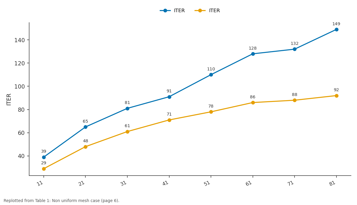
ITER and ITER: 11 vs 21 vs 31 vs 41 vs 51
Replotted from Table 1 (page 6) of the original paper. Every bar is the paper's own table value.
View source evidence ↗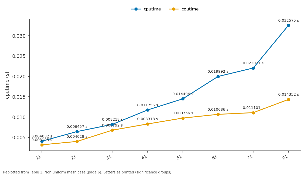
cputime and cputime: 11 vs 21 vs 31 vs 41 vs 51
Replotted from Table 1 (page 6) of the original paper. Every bar is the paper's own table value.
View source evidence ↗Figures & tables
From the original paper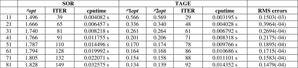 Table 1
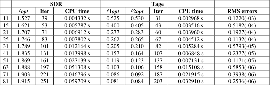 Table 2
Introduction
Despite the fact that splines can be of any degree, cubic splines have the most norms by a long shot. A cubic spline is one that is formed up of piecewise third-engineer polynomials and has a lot of control points. At the endpoints of every polynomial, the second subordinate is usually set to zero, as this provides a breaking point condition that completes the game plan of conditions. This results in a "natural" cubic spline with an acceptable tri-corner to corner structure that can be properly dealt with to obtain the polynomial coefficients. However, this option isn't the only one available and other breaking point criteria could be used as well. Rajashekhar et al. (2017) [5] studied the Efficient Numerical Solution for Seventh Order Differential Equation by Using Septic B-Spline Collocation Method with Non-Uniform Length. Busyra et al. (2021) [4] delivered a brand new cubic B-spline (CBS) approximation approach to resolve linear two-factor boundary cost problems (BVPs). This approach is primarily based totally on cubic B-spline foundation capabilities with a brand new approximation for the second-order derivative. The numerical outcomes had been as compared with the least squares approach, finite distinction approach, finite detail approach, finite extent approach, B-spline interpolation approach, prolonged cubic B-spline interpolation approach and the precise solution. Khalid et al. (2019) [2] suggested a computational model based on the cubic B-spline method for solving linear 6th order BVPs that arise in astronomy. The boundary problem is transformed into a system of linear equations using the approach specified. The technique we will build in this work is not only an approximation solution of the 6th order BVPs using cubic B-spline, but it also explains the estimated derivatives of the analytic solution from 1st order to 6th order. This unique technique is second order convergent and has a lower computational cost than many existing strategies. The findings are shown in error tables and graphs, and they are compared to previous research findings. Nazir et al. (2019) [2] Using the seventh-degree B-Spline function, we provide a numerical method for addressing the boundary value problem of The Linear Seventh Ordinary Boundary Value Problem. The formulation is based on specific terms of the seventh-order boundary value problem's order. The Collocation B-spline approach is formulated as an approximation solution, and we gain Septic B-Spline formulation. We use the proposed method to solve a seventh-order boundary value problem, and the results indicate that approximate and exact solutions agree.
The numerical method given is helpful for solving high order boundary value issues since it produces low absolute errors. A broad conclusion has been included at the end. Manan et al. (2018) [8] . An algorithm to solve 3rd order boundary value problem is focused in this paper which is 8-point approximating scheme. It concludes the results with stability and convergence that is evaluated with the illustration of numerical example. This paper also contains the analysis of approximation properties for the mentioned collocation algorithm. Heilat and Hailat (2020) [1] prolonged cubic B-spline approach for fixing a gadget of nonlinear second-order boundary price problems. A quasi linearization method is used and the mistake estimate is acquired. The accuracy of the approach relies upon on loose parameters. We practice the approach on 4 examples and the outcomes which acquired the use of prolonged cubic B-spline suggest that the approach is green and accurate. Siraj-ul-Islam et al. (2006) [7] studied the Quadratic Non-Polynomial Spline Approach to the Solution of a System of Second-Order Boundary-Value Problems. Tahir et al. (2019) [3] proposed a new quantic B-spline approximation technique for solving the Boussinesq problem numerically. Two test examples are used to confirm the new scheme's performance and accuracy. The computational results are shown to be superior to current numerical techniques on the subject. Mustafa et al. (2017) [9] the solution of non-linear fourth order boundary value problems involving ordinary differential equations, this work provides an iterative collocation numerical technique based on interpolating subdivision schemes. The technique converges to a smooth approximate solution of the non-linear fourth order boundary value problem, according to numerical evidence. The approach's convergence is also examined. The main goal of this paper is to look into and find applications for subdivision systems in physics and engineering. Pervaiz et al. (2014) [10] developed a numerical technique for solving sixth order boundary value problems (BVPs). The sixth order BVPs were first reduced to a system of second order BVPs. The system of second order BVPs was then reduced to a system of linear algebraic equations with boundary conditions using non-polynomial cubic spline and finite difference approximations. The strategy was tested on three test issues with step sizes of h = 1/5 and h = 1/10 to see if it was useful. Tables and graphs have been used to demonstrate the method's accuracy in achieving the exact solution. Shahid S. Siddiq et al. (2007) [11] . The numerical solution of the sixth-order linear, special case boundary value problem is done using the septic spline. The definition of a septic spline is given with end conditions that are consistent with the sixth-order boundary value problem. The solution and their higher-order derivatives are approximated using the algorithm proposed. It has also been demonstrated that the approach is second-order convergent. For numerical illustrations of the developed approach, three instances are studied. The approach described in this study is compared to that produced in [M. El-Gamel, J.R. Cannon, J. Latour, A.I. Zayed, Sinc-Galerkin method for solving linear sixth order boundaryvalue problems, Mathematics of Computation 73, 247 (2003) 1325-1343], and it is found to be superior.
Cube Spline Formulation
We discretize arrangement locale [0, 1] with non-uniform work so such an extent that 0 = 𝑥 0 < 𝑥 1 … … < 𝑥 𝑁+1 = 1. Our method includes three matrix focuses
, 𝑖 = 1(1)𝑁 + 1 and the work extent is 𝜎 𝐾 = (ℎ 𝑘+1 /ℎ 𝑘 ) > 0. Right when 𝜎 𝐾 = 1, at that point it decreases to constant mesh case. Let the right estimations of 𝑢(𝑥) at matrix point 𝑥 𝑘 be implied by 𝑈 𝐾 = 𝑢(𝑥 𝑘 ) and 𝑢 𝑘 be the rough estimations of 𝑈 𝐾 . At the matrix point 𝑥 𝑘 , let us show
All through our trade, we consider that our answer contains odd number of inside grid points, for instance 𝑁 as odd. We initially build up a numerical method for evaluating integral ∫ 𝐺(𝑥)𝑑𝑥 1 0
Where 𝑏 -1 , 𝑏 0 , 𝑏 1 are boundaries to be chose and at point 𝑥 𝑘 , we show 𝐺 𝑘 = 𝐺(𝑥 𝑘 ) Further, we may compose utilizing Taylor's expansion
Using ( 4)-( 5), comparing both sides of (1), we get
Accordingly one might be compose third request integral formula (2) in variable mesh frame as
Note that coefficients related with right hand side of ( 9) are sure, assuming likewise, for example, 2 -𝜎 𝑘 > 0 & 2𝜎 𝑘 -1 > 0 i.e
Can be found by the reiterated use of formula (2), when N is odd. Directly we analyzed the variable work cubic spline strategy for differential con. (3). Cubic spline interjecting polynomial of degree three then [𝑥 𝑘-1, 𝑥 𝑘 ] can be made as
Which satisfies the accompanying with conditions in each subinterval[𝑥 𝑘-1, 𝑥 𝑘 ], 𝑘 = 1(1)𝑁 + 1, 𝑆(𝑥), coincides with a polynomial of degree three, 𝑆(𝑥) ∈ 𝐶 2 [0,1] and 𝑆(𝑥 𝑘 ) = 𝑢 𝑘 , 𝑘 = 0(1)𝑁 + 1
Where 𝑀 𝑘 = 𝑢 " (𝑥 𝑘 ) = 𝜓(𝑥 𝑘 , 𝑢(𝑥 𝑘 ), 𝑢 ′ (𝑥 𝑘 )) ≡ 𝑠𝑎𝑦
The approximation (15) to be of, coefficient of must be zero;
Finally, by assistance of ( 16) -( 18), one can assess
𝜓 ̂𝑘 = 𝜓(𝑥 𝑘 , 𝑈 𝑘 , 𝑈 ̂𝑘 𝑙 ) = 𝜓 𝑘 + 𝑂(ℎ 𝑘 3 )
By then the cubic spline approximation of precision of 𝑂(ℎ 𝑘 3 )for given integral differential conditions (1) may be created as
[𝑃 𝑘 𝛹 ̂𝑘+1 + 𝑄 𝑘 𝛹 ̂𝑘 + 𝑅 𝑘 𝛹 ̂𝑘-1 ] + 𝑇 ̂𝑘, 𝑘 = 1(1)𝑁
For convergence of the distinction method, coefficients on right hand side of conditions (19) must be sure, i.e., one has the condition
forced on our choice of mesh proportion parameter. Note that the limit esteems are given by 𝑢 0 = 𝑈 0 = 𝑎 0 & 𝑢 𝑁+1 = 𝑈 𝑁+1 = 𝑎 1 . Joining the limit esteems in numerical approximation (19), we can procure a tri-diagonal framework of equations. If the differential equation is linear, one can comprehend the framework by AGE iterative strategy and for nonlinear case, one can compared the framework by Newton-AGE iterative method.
Application of Newton TAGE Method
Next we talk about the utilization of Newton-TAGE iterative strategy for nonlinear difference conditions (19). Dismissing the mistake term, one may re-compose nonlinear difference equation (19) as
The Jacobian of ∅(𝑢) may be spoken as
is any halfway vector. We characterize
By then a two-advance explicit Newton-TAGE strategy may be formed as
(𝑇 2 + 𝜌 2 𝐼)∆𝑣 (𝑠+1) = -∅(𝑢 (𝑠) ) -(𝑇 1 + 𝜌 2 𝐼)∆𝑣 (𝑠) , s≥ 0
Where 𝛥𝑣 is any moderate vector. Since the matrices (𝑇 1 + 𝜌 1 𝐼) & (𝑇 2 + 𝜌 2 𝐼)comprise of (2×2) sub-matrices, hereafter they are successfully invertible and from ( 23) & (24), we get
Finally, by the assistance of ( 25)-( 26), from (23) one can secure numerical solution at (𝑠 + 1) th iteration. For intermingling, it is required that one pick 𝑢 (0) "close" to solution u.
Results and Conclusions
In this section, we dealt with the following with two benchmark issues on both uniform and non-uniform work whose correct arrangement is known to us, and we differentiated the outcomes and the corresponding successive over relaxation and Newton-SOR approach. For uniform work, one take 𝜎 𝑘 = 𝜎 = 1 7 for non-uniform mesh, one take 𝜎 𝑘 = 𝜎 = 𝑎 constant≠ 1, 𝑘 = 1(1)𝑁 + 1. By then estimation of first mesh isolating on left is given by
Thusly, for non-uniform mesh, given the assessment of 𝑁, we can figure initial step length ℎ 1 from above associated and rest of the work is likewise controlled by h 𝑘+1 = 𝜎ℎ 𝑘 , 𝑘 = 1(1)𝑁. Such a constringent isn't relevant to uniform work case. By taking 𝜎 𝑘 = 𝜎 = 1, one can apply the strategies clearly to uniform mesh. All calculations were finished utilizing MATLAB. In all cases, one has considered 𝑢 (0) = 0 and the iterations were stopped when the preeminent blunder |𝑢 (𝑠+1) -𝑢 (𝑠) | ≤ 10 (28) 0 < 𝑥 < 1, 0 < 𝑠 < 1
The limit esteems are given by (0) = 1, 𝑢(1) = 𝑒. The right arrangement of problem is given by (𝑥) = 𝑒 𝑥
The boundary estimations are given by 𝑢(0) = 0, 𝑢(1) = 𝑐𝑜𝑠ℎ (1).
The solution of problem is given by (𝑥) = 𝑥 2 𝑐𝑜𝑠ℎ 𝑥. The RMS errors, optimal values (𝜌 𝑜𝑝𝑡 , 𝜌 1𝑜𝑝𝑡 , 𝜌 2𝑜𝑝𝑡 ) of relaxation parameters & number of iterations both for Newton-TAGE & Newton-SOR methods for non-uniform and uniform mesh case are tabulated in Table 2(A) for (𝛼, 𝜎) = (0, 0.8).
| — | SOR | — | — | Tage | — | — | — | — |
|---|---|---|---|---|---|---|---|---|
| opt | Iter | CPU time | 1opt | 2opt | Iter | CPU time | RMS errors | |
| 11 | 1.527 | 39 | 0.004332 s | 0.525 | 0.530 | 31 | 0.002968 s | 0.1220(-03) |
| 15 | 1.621 | 53 | 0.005787 s | 0.400 | 0.405 | 43 | 0.003516 s | 0.5182(-04) |
| 21 | 1.707 | 71 | 0.006912 s | 0.277 | 0.283 | 60 | 0.003960 s | 0.1927(-04) |
| 25 | 1.746 | 83 | 0.007802 s | 0.262 | 0.265 | 67 | 0.004512 s | 0.1132(-04) |
| 31 | 1.789 | 101 | 0.012164 s | 0.205 | 0.210 | 82 | 0.005284 s | 0.5793(-05) |
| 41 | 1.835 | 131 | 0.013998 s | 0.157 | 0.164 | 107 | 0.006848 s | 0.2377(-05) |
| 51 | 1.869 | 161 | 0.027139 s | 0.119 | 0.123 | 137 | 0.007131 s | 0.1171(-05) |
| 63 | 1.888 | 197 | 0.051308 s | 0.103 | 0.106 | 158 | 0.015108 s | 0.5853(-06) |
| 71 | 1.903 | 221 | 0.046796 s | 0.086 | 0.092 | 187 | 0.021915 s | 0.3938(-06) |
| 81 | 1.915 | 251 | 0.059709 s | 0.081 | 0.084 | 203 | 0.032910 s | 0.2536(-06) |
Table text extracted from the original PDF; superscript letters are shown inline. The original table image is below.
View original table image
Example-1:
The RMS Errors (Non uniform mesh case) Example-2: The RMS Errors (uniform mesh case)
Conclusion
Another three-point variable work approach based on cubic spline surmise for the game plan of second request nonlinear twopoint limit respect issue with absolutely healthy driving cutoff points has been demonstrated. All things considered, the recommended system for 𝜎 𝐾 = 1 is monitored to see whether it reduces to an anticipated work approach for precision of request four. When the number of internal framework explanations behind the course of action space is unusual, the recommended technique is applicable. Both immediate and nonlinear difficulties with lone coefficients, as well as driving cutoff points in critical packaging are well-suited to the approach. The application of TAGE and Newton-TAGE techniques demonstrates the power of differentiating SOR and Newton-SOR procedures in terms of cycle count. The offered solutions could be applied to multidimensional situations.
Figures and tables from the paper
| — | SOR | — | — | TAGE | — | — | — | — |
|---|---|---|---|---|---|---|---|---|
| opt | ITER | cputime | 1opt | 2opt | ITER | cputime | RMS errors | |
| 11 | 1.496 | 39 | 0.004082 s | 0.566 | 0.569 | 29 | 0.003195 s | 0.1503(-03) |
| 21 | 1.666 | 65 | 0.006457 s | 0.336 | 0.340 | 48 | 0.004028 s | 0.3964(-04) |
| 31 | 1.740 | 81 | 0.008218 s | 0.261 | 0.264 | 61 | 0.006792 s | 0.2694(-04) |
| 41 | 1.766 | 91 | 0.011755 s | 0.201 | 0.206 | 71 | 0.008318 s | 0.2175(-04) |
| 51 | 1.787 | 110 | 0.014496 s | 0.170 | 0.174 | 78 | 0.009766 s | 0.1895(-04) |
| 61 | 1.794 | 128 | 0.019992 s | 0.164 | 0.168 | 86 | 0.010686 s | 0.1715(-04) |
| 71 | 1.805 | 132 | 0.022071 s | 0.154 | 0.158 | 88 | 0.011101 s | 0.1583(-04) |
| 81 | 1.828 | 149 | 0.032575 s | 0.134 | 0.139 | 92 | 0.014352 s | 0.1479(-04) |
Table text extracted from the original PDF; superscript letters are shown inline. The original table image is below.
View original table image
References
11 in the original paper- Ahmed Salem Heilat, Reyadh Sallem Hailat. Extended cubic B-spline method for solving a system of nonlinear second-order boundary value problems. J Math. Comput. Sci. 2020;21(3):231-42.
- Khalid A, Naeem MN, Agarwal P, et al. Numerical approximation for the solution of linear sixth order boundary value problems by cubic B-spline. Adv Differ Equ. 2019;2019(1):1-6. https://doi.org/10.1186/s13662-019-2385-9.
- Tahir Nazir, Muhammad Abbas, Muhammad Kashif Iqbal. A new quintic B-spline approximation for numerical treatment of Boussinesq equation. J Math. Comput. Sci. 2019;20(1):30-42.
- Busyra Latif, Samsul Ariffin Abdul Karim, Ishak Hashim. New Cubic B-Spline Approximation for Solving Linear Two-Point Boundary-Value Problems. Mathematics. 2021;9(11):1250.
- Rajashekhar Reddy Y. Efficient Numerical Solution for Seventh Order Differential Equation by Using Septic B-Spline Collocation Method with Non-Uniform Length. Global Journal of Pure and Applied Mathematics. 2017;13(7):3543-3548.
- Nazir T, Abbas M, Iqbal MK. A New Quintic B-Spline Approximation for Numerical Treatment of Business q Equation. Journal of Mathematics and Computer Science. 2020;20(1):30-42. https://doi.org/10.22436/jmcs.020.01.04
- Siraj-ul-Islam MA, Noor Tirmizi IA, Khan MA. Quadratic Non-Polynomial Spline Approach to the Solution of a System of Second-Order Boundary-Value Problems, Applied Mathematics and Computation. 2006 August;179(1):153-160. Doi: 10.1016/j.amc.2005.11.091.
- Manan SA, Ghaffar A, Rizwan M, Rahman G, Kanwal G. A subdivision approach to the approximate solution of 3rd order boundary value problem. Commun. Math. Appl. 2018;9(4):499-512.
- Mustafa G, Abbas M, Ejaz ST, Ismail AIM, Khan F. A numerical approach based on subdivision schemes for solving nonlinear fourth order boundary value problems. J. Comput. Anal. Appl. 2017;23(4):607-623.
- Pervaiz A, Ahmad A, Zafar Z, Ahmad M. Numerical solution of sixth order BVPs by applying non-polynomial spline method. Pak. J Sci. 2014;66(2):110-116.
- Siddiqi SS, Akram G. Septic spline solutions of sixth-order boundary value problems. J Comput. Appl. Math. 2008;215(1):288-301.