
Research article · 2021 · Full text
International Journal of Statistics and Applied MathematicsAnalysis of S&P 500 stocks: Long-term vs short-term investment
Volume 6(6) · Pages 158–164 · DOI: 10.22271/maths.2021.v6.i6b.761 ↗
Research areasComplex Systems and Time Series AnalysisStock Market Forecasting Methods
Abstract
Author-writtenThis paper is concerned with analyzing the stocks in the Standard & Poors 500 Index that potentially yield high returns. To achieve this goal, historical stock prices and their corresponding simple moving averages are used together to capture the stock trend directions. When the time series of the stock crosses over its corresponding simple moving average line from below (or above), it indicates an up (or down) trend signal and a buy (or sell) is initiated. A trading strategy consisting of these buying and selling indicators is implemented. Simple moving averages of various lengths are constructed and employed in order to maximize the return for each stock. The results suggest that long-term trading can potentially yield high returns and short-term trading generally perform poorly.
Summary
Source-checkedPlain-language reading of the full paper, prepared with AI and checked against the text. Each point links to the authors' own words.
Why it matters
- Daily stock price time series are generally categorized into three types: geometric Brownian motion, mean-reverting processes, or trend-following processes. View evidence ↗
- Moving averages are widely used technical indicators in trading due to their simplicity and ease of application. View evidence ↗
- The study focuses on using a simple moving average (SMA) method to identify high-return stocks within the S&P 500 Index rather than creating new trading strategies. View evidence ↗
The question
- The primary objective of the research is to analyze which stocks in the S&P 500 Index have the potential to yield high returns. View evidence ↗
What they did
- The researchers analyzed daily adjusted prices for 478 S&P 500 companies over a six-year period from January 2, 2014, to December 27, 2019, totaling 1,508 observations. View evidence ↗
- The trading strategy initiates a 'buy' when the stock price crosses above the SMA and a 'sell' when it crosses below the SMA. View evidence ↗
- To maximize returns for each stock, the study tested SMA lengths ranging from 5 to 500 days in increments of 5. View evidence ↗
What they found
- The top 50 stocks achieved an average mean percentage return of 43.5% per round-trip trade, with an average of 4 trades over six years. View evidence ↗
- The bottom 50 stocks performed poorly, gaining at most 0.2% per round-trip trade on average, despite a high frequency of approximately 107 trades over six years. View evidence ↗
- The data indicates that long-term investment strategies, characterized by fewer round-trip trades, generally perform better than short-term strategies. View evidence ↗
- Long-term investment does not guarantee success, as some stocks with 6 or fewer round-trip trades still yielded mean percentage returns below 10%. View evidence ↗
What it means
- The authors conclude that the SMA method successfully identified ten S&P 500 stocks (including NVDA, AMD, and GE) that potentially generate high returns through long-term investing. View evidence ↗
- A limitation of the study is that the implementation did not account for transaction costs, which would likely further reduce the returns of short-term trading. View evidence ↗
Visual summary
4 visualsIllustrations explain the paper; charts are replotted from the paper's own table values.

SMA Crossover Logic
AI-generated conceptual illustration (A digital financial candlestick chart on a dark computer screen). It explains the idea and does not show study data.
View source evidence ↗
Return vs Trade Frequency
AI-generated conceptual illustration (A digital representation of a stock market portfolio). It explains the idea and does not show study data.
View source evidence ↗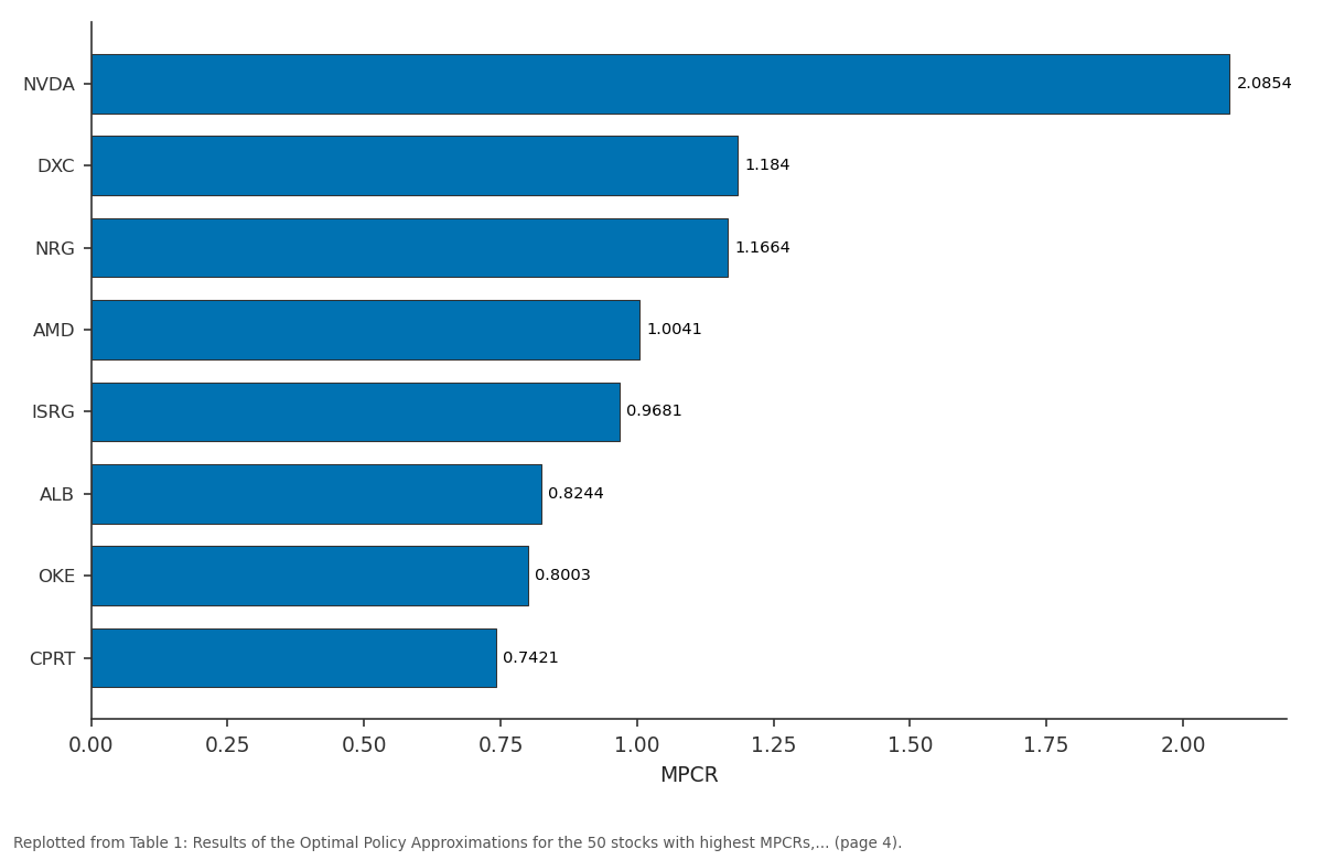
MPCR: NVDA vs DXC vs NRG vs AMD vs ISRG
Replotted from Table 1 (page 4) of the original paper. Every bar is the paper's own table value.
View source evidence ↗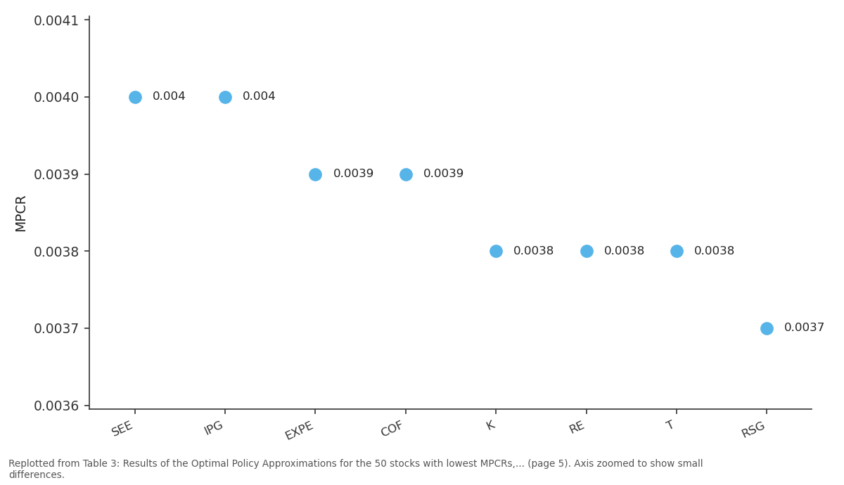
MPCR: SEE vs IPG vs EXPE vs COF vs K
Replotted from Table 3 (page 5) of the original paper. Every bar is the paper's own table value.
View source evidence ↗Figures & tables
From the original paper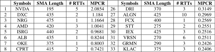 Table 1
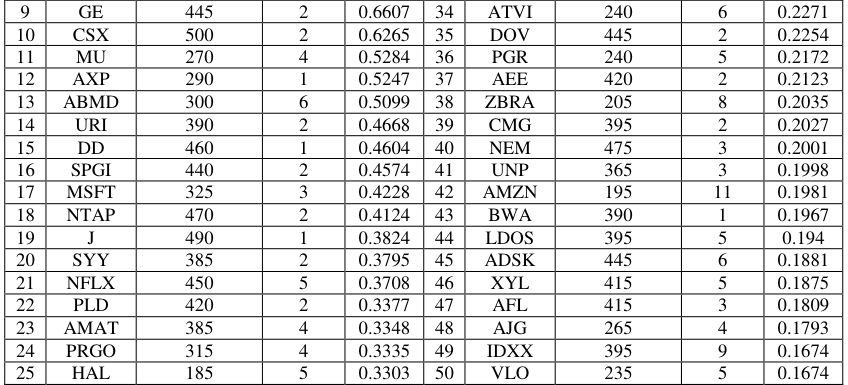 Table 2
 Table 2
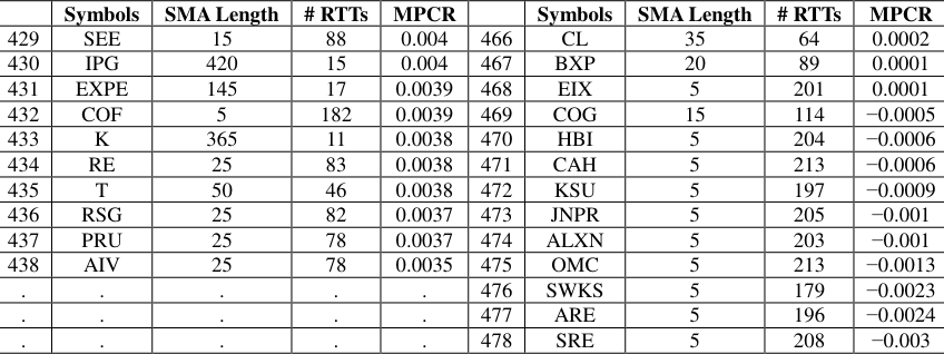 Table 3
 Table 4
 Table 5
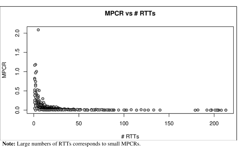 Figure 1
Introduction
A time series of daily stock prices can be classified as a geometric Brownian motion (GBM), a mean-reverting process (MR), or a trend-following process (TR). Trading strategies have been developed for each type of processes. A GBM is technically a Markov process. This means the stock prices follow a random walk. Merhi and Zervos (2007) [10] studied an investment capacity expansion/reduction problem following a dynamic programming approach under a GBM market model. In addition, Guo and Zhang (2005) [3] studied the optimal selling rule under a model with switching GBM. Using a smooth-fit technique, they obtained the optimal threshold levels by solving a set of algebraic equations. A MR refers to a time series that displays a tendency to revert to its historical mean value. Such a time series is referred to as an Ornstein-Uhlenbeck process. The mean-reverting property of a time series can be exploited in order to produce profitable trading strategies. A common strategy in mean-reversion trading is to buy low and sell high. For example, Luu et al. (2018a) [8] focused on a threshold type policy and developed a method that was easy to implement in practice. They formulated the optimal trading problem in terms of a sequence of optimal stopping times. The optimal threshold levels could be obtained by solving quasialgebraic equations. Recently, Luu et al. (2018b) [9] developed pairs trading strategies under both mean-reverting and geometric Brownian motion models. They showed that pairs trading ideas were more general and not necessary to be cast under a mean-reverting framework. A TR is assumed to continue to move in the same direction as the current trend. Dai et al. (2010) [1] developed a trend-following rule based on a conditional probability indicator. They showed that the optimal trading rule can be determined by two threshold curves which can be obtained by solving the associated Hamilton-Jacobi-Bellman equations. A similar idea was developed following a confidence interval approach by Iwarere and Barmish (2010) [4] . Trading strategies have been studied for many years and never before have stock investors heavily relied on them. An effective strategy also needs appropriate stocks to work well. In this paper, instead of developing trading strategies, a simple moving average method is implemented to identify stocks in the Standard & Poor's 500 Index that potentially yield high returns. The results show that high returns only exist in long-term trading. In addition, longterm investment can fail in many stocks and so do short-term trading in general.
Simple Moving Average (SMA)
We use simple moving averages to identify trends in stocks. A simple moving average shows the average price over a certain period of time. As prices change, the corresponding simple moving averages generally either increase or decrease. A SMA is calculated by adding prices over a given number of periods, then dividing the sum by the number of periods or length. Each time a new period occurs, the moving average moves forward dropping its first data point and adding the newest one (Learn Price Action, 2020) [6] . For a time series of length N periods: x1, x2, . . . , xN, a simple moving average of length n or n-day SMA is a time series of the form:
In this paper, historical daily adjusted prices of a stock and its corresponding simple moving averages are used together to capture the stock trend directions. When the time series of the stock crosses over its corresponding simple moving average line from below, it indicates an uptrend signal and a buy is initiated. On the other hand, when the time series of the stock crosses its corresponding simple moving average line from above, it indicates a down trend signal and a sell is initiated (Mitchell, 2020) [11] . A trading strategy consisting of these buying and selling indicators within a considered time frame is implemented. The length of a SMA can play a significant role in the effectiveness of the method. A SMA with a short length reacts more quickly to price changes than that with a long length. For example, a 10-day SMA tracks the original prices more closely than a corresponding 100-day SMA does (Kenton, 2018) [5] . So it is possible to adjust the lengths so that the SMAs generate more reliable signals for the data. This may help create better future signals. While Forex trading commonly uses moving averages over lengths of 10, 50, 100, and 200 (Lioudis, 2020) [7] , we use a bigger range of lengths in order to "maximize" the return for each stock. SMAs with lengths of 5, 10, 15, . . . , and 500 are employed in this paper.
Policy and Return
Almost all trading strategies involve optimizing the return: maximizing the return or profit. The returns investors can expect to receive in the future depend on what actions they will take. For a time series x of a stock's daily adjusted prices: x1, x2, . . ., xN, where the dates are indexed as 1, 2, . . . , N, a sequence of buying and selling actions at times (b1, s1), (b2, s2), . . ., within the time frame of the time series, is called a policy π x . In a policy obtained from a SMA, b1 (or s1) is the time where the stock crosses over the SMA from below (or above respectively) for the first time. Similarly, bn (or sn) is the time where the stock crosses over the SMA from below (or above respectively) for the n th times, where b1 < s1 < b2 < s2 < •••. Buying a stock at time bi and selling it later at time si is called a round-trip trade (RTT). Given a time series x and an n-day SMA, suppose the corresponding policy π x,n contains a sequence of buying and selling actions at times (b1, s1), (b2, s2 ), . . . , (bK , sK). Then 1. The percentage return (PCR) of the RTT at (bi, si) can be computed by
2. The mean percentage return (MPCR) of π x,n can be computed by
𝐾𝐾
We define SMA(x, n) the time series representing the n-day SMA of the time series x.
We define MEAN(z) the arithmetic mean of z if z is a list of real numbers or the MPCR of z if z is a policy of a time series. Let P x be the set of all policies of the time series x. An optimal policy π o,x , which gives the maximum value of MPCRs of the time series, can be defined by
Optimal Policy Approximation with an n-day SMA
Pseudocode for obtaining a policy with an n-day SMA is shown in Algorithm 1. The function GetPolicy(x, n) is assumed to take a time series x and a length n of a SMA, and return the corresponding policy π x,n .
Algorithm 1: GetPolicy(x, n) for obtaining a policy with an n-day SMA Input: x: a time series of length N. n: the length of a simple moving average. Output: The policy π x,n containing a list of buying and selling times. Line 1: Calculate the n-day SMA for the time series x and store the result in y. Line 2: Loop through all the time indices to compare the values of the n-day SMA and their corresponding values of x at each time. Note that an n-day SMA starts at time n. Line 3 and 4: If the value of x is above that of its simple moving average at time i then assign the signal variable sigi to 1. Line 5 and 6: If the value of x is below that of its simple moving average at time i then assign the signal variable sigi to -1. Line 7 and 8: If the value of x is equal to that of its simple moving average at time i then assign the signal variable sigi to 0 (the two lines intersect at i). Line 9: Obtain all the time indices where x crosses over its simple moving average from below and store them in b. These are the buy signals. Line 10: Obtain all the time indices where x crosses over its simple moving average from above and store them in s. These are the sell signals. Line 11: Return the policy of x corresponding to the n-day SMA.
Next pseudocode for an optimal policy approximation with n-day SMAs is presented in Algorithm 2. The algorithm is assumed to take the set of stocks and the set of lengths used in SMAs, and returns an optimal policy approximation π o,x for each stock x and the corresponding SMA's length n o,x and MPCR Line 1: Loop through each stock x in S. Line 2, 3, and 4: Initiate the values for the optimal policy for each stock x. MPCR o,x is assigned to a small value so that it can be updated later. Line 5: For each stock x, loop through the list of SMAs' lengths to search for a n-day SMA which gives a "best" approximation of the optimal policy. Line 6, 7, and 8: Obtain the policy for x corresponding to the n-day SMA, and store the buy signals in b and the sell signals in s. Note that b and s may have different lengths at this point. Line 9: Check if there is any round-trip trade to calculate the MPCR x,n . Line 10 through 15: Equalize the lengths of b and s, and store the common length in K. If there are more buy signals than sell signals, the last buy signal will be dropped. On the other hand, if there are more sell signals than buy signals, the first sell signal will be dropped. Note that b and s are adjusted to have the same indices: 1, 2, . . ., K. Line 16: Calculate each percentage return (xsi -xbi)/xbi for each round-trip trade, and store the values in the list PCR x,n . Line 17: Calculate the mean percentage return for the current n-day SMA. Line 18 through 21: Update the approximation of the optimal policy for x if a better policy is found.
Result and Discussion
The algorithm Optimal Policy Approximation with n-day SMAs are implemented using the R programming language with the following input: S = the set of all 478 stocks of S&P 500 as described above. L = {5, 10, 15, . . . , 500}: the set of SMA lengths. The output of the algorithm is the approximation of the optimal policy for each stock in S. Each row of Table 3 and Table 4 lists the stock and its summary of the optimal policy approximation containing the corresponding length of the simple moving average (SMA length), the number of round-trip trades (# RTTs), and the mean percentage return (MPCR). As can be seen from Table 1 and Table 2, it is possible to gain 43.5% per round-trip trade on average for the top 50 stocks, and there are approximately 4 round-trip trades on average over the six-year period. Moreover, the result is very impressive for the top 10 stocks. In particular, it is possible to gain up to 100.6% per round-trip trade on average and there are approximately 2 roundtrip trades over the six-year period.
| — | SMA Length | # TTs | MPCR |
|---|---|---|---|
| Avg. bottom 50 | 54.8 | 107.28 | 0.001502 |
| Avg. bottom 10 | 6 | 193.2 | −0.00136 |
Table text extracted from the original PDF; superscript letters are shown inline. The original table image is below.
View original table image
| — | Symbols | SMA Length | # RTTs | MPCR | — | Symbols | SMA Length | # RTTs | MPCR |
|---|---|---|---|---|---|---|---|---|---|
| 429 | SEE | 15 | 88 | 0.004 | 466 | CL | 35 | 64 | 0.0002 |
| 430 | IPG | 420 | 15 | 0.004 | 467 | BXP | 20 | 89 | 0.0001 |
| 431 | EXPE | 145 | 17 | 0.0039 | 468 | EIX | 5 | 201 | 0.0001 |
| 432 | COF | 5 | 182 | 0.0039 | 469 | COG | 15 | 114 | −0.0005 |
| 433 | K | 365 | 11 | 0.0038 | 470 | HBI | 5 | 204 | −0.0006 |
| 434 | RE | 25 | 83 | 0.0038 | 471 | CAH | 5 | 213 | −0.0006 |
| 435 | T | 50 | 46 | 0.0038 | 472 | KSU | 5 | 197 | −0.0009 |
| 436 | RSG | 25 | 82 | 0.0037 | 473 | JNPR | 5 | 205 | −0.001 |
| 437 | PRU | 25 | 78 | 0.0037 | 474 | ALXN | 5 | 203 | −0.001 |
| 438 | AIV | 25 | 78 | 0.0035 | 475 | OMC | 5 | 213 | −0.0013 |
| . | . | . | . | . | 476 | SWKS | 5 | 179 | −0.0023 |
| . | . | . | . | . | 477 | ARE | 5 | 196 | −0.0024 |
| . | . | . | . | . | 478 | SRE | 5 | 208 | −0.003 |
Table text extracted from the original PDF; superscript letters are shown inline. The original table image is below.
View original table image
| — | SMA Length | # TTs | MPCR |
|---|---|---|---|
| Avg. Top 50 | 369.5 | 3.52 | 0.43542 |
| Avg. Top 50 | 413.5 | 2.1 | 1.0062 |
Table text extracted from the original PDF; superscript letters are shown inline. The original table image is below.
View original table image
| 9 | GE | 445 | 2 | 0.6607 | 34 | ATVI | 240 | 6 | 0.2271 |
|---|---|---|---|---|---|---|---|---|---|
| 10 | CSX | 500 | 2 | 0.6265 | 35 | DOV | 445 | 2 | 0.2254 |
| 11 | MU | 270 | 4 | 0.5284 | 36 | PGR | 240 | 5 | 0.2172 |
| 12 | AXP | 290 | 1 | 0.5247 | 37 | AEE | 420 | 2 | 0.2123 |
| 13 | ABMD | 300 | 6 | 0.5099 | 38 | ZBRA | 205 | 8 | 0.2035 |
| 14 | URI | 390 | 2 | 0.4668 | 39 | CMG | 395 | 2 | 0.2027 |
| 15 | DD | 460 | 1 | 0.4604 | 40 | NEM | 475 | 3 | 0.2001 |
| 16 | SPGI | 440 | 2 | 0.4574 | 41 | UNP | 365 | 3 | 0.1998 |
| 17 | MSFT | 325 | 3 | 0.4228 | 42 | AMZN | 195 | 11 | 0.1981 |
| 18 | NTAP | 470 | 2 | 0.4124 | 43 | BWA | 390 | 1 | 0.1967 |
| 19 | J | 490 | 1 | 0.3824 | 44 | LDOS | 395 | 5 | 0.194 |
| 20 | SYY | 385 | 2 | 0.3795 | 45 | ADSK | 445 | 6 | 0.1881 |
| 21 | NFLX | 450 | 5 | 0.3708 | 46 | XYL | 415 | 5 | 0.1875 |
| 22 | PLD | 420 | 2 | 0.3377 | 47 | AFL | 415 | 3 | 0.1809 |
| 23 | AMAT | 385 | 4 | 0.3348 | 48 | AJG | 265 | 4 | 0.1793 |
| 24 | PRGO | 315 | 4 | 0.3335 | 49 | IDXX | 395 | 9 | 0.1674 |
| 25 | HAL | 185 | 5 | 0.3303 | 50 | VLO | 235 | 5 | 0.1674 |
Table text extracted from the original PDF; superscript letters are shown inline. The original table image is below.
View original table image
| — | Symbols | SMA Length | # RTTs | MPCR | — | Symbols | SMA Length | # RTTs | MPCR |
|---|---|---|---|---|---|---|---|---|---|
| 1 | NVDA | 195 | 5 | 2.0854 | 26 | DRI | 370 | 3 | 0.3149 |
| 2 | DXC | 435 | 2 | 1.184 | 27 | ALGN | 425 | 10 | 0.2969 |
| 3 | NRG | 475 | 1 | 1.1664 | 28 | FCX | 400 | 1 | 0.2569 |
| 4 | AMD | 420 | 3 | 1.0041 | 29 | STT | 275 | 2 | 0.2551 |
| 5 | ISRG | 440 | 2 | 0.9681 | 30 | IEX | 425 | 3 | 0.2516 |
| 6 | ALB | 435 | 1 | 0.8244 | 31 | VRSN | 270 | 6 | 0.2511 |
| 7 | OKE | 375 | 1 | 0.8003 | 32 | GRMN | 290 | 3 | 0.2426 |
| 8 | CPRT | 415 | 2 | 0.7421 | 33 | KLAC | 375 | 3 | 0.2406 |
Table text extracted from the original PDF; superscript letters are shown inline. The original table image is below.
View original table image
Note:
The values in the first and second rows are the averages of each column of SMA length, #RTTs, and MPCR using all 50 rows and the first 10 rows from Table 3 respectively.
Table 3 and Table 4 show that one can gain at most 0.2% per round-trip trade on average for the bottom 50 stocks in Table 3, and there are approximately 107 round-trip trades on average over the six-year period. Moreover, the performance is very poor for the bottom 10 stocks. Specifically, one can lose at least 0.1% per round-trip trade on average and there are approximately 193 roundtrip trades over the six-year period. These results suggest that long-term investment (small number of round-trip trades) performs better. Moreover, the top 10 stocks, where the numbers of round-trip trades are between 1 and 5, can possibly yield high returns in the long run. The values in the first and second rows are the averages of each column of SMA length, # RTTs, and MPCR using all 50 rows and the last 10 rows from Exhibit 8 respectively.
However, not all long-term investments can generate good results. For example, Table 5 lists stocks with small numbers of RTTs (at most 6), yet the corresponding MPCRs are less than 10%. The scatter plot in Figure 1 confirms that high returns only exist in long-term investing in S&P 500, while short-term investing (large number of round-trip trades) generally yields poor result. As the number of round-trip trades increases, the MPCR is very close to zero.
| Symbols | SMA Length | #RTTs | MPCR | Symbols | SMA Length | # RTTs | MPCR |
|---|---|---|---|---|---|---|---|
| NLSN | 445 | 2 | 0.0008 | TPR | 500 | 4 | 0.0566 |
| BEN | 295 | 6 | 0.0058 | TXT | 495 | 5 | 0.0604 |
| ETR | 490 | 6 | 0.0071 | TSCO | 420 | 3 | 0.0612 |
| SPG | 400 | 6 | 0.0146 | TAP | 410 | 4 | 0.0633 |
| EMN | 405 | 6 | 0.0251 | LIN | 355 | 5 | 0.0682 |
Table text extracted from the original PDF; superscript letters are shown inline. The original table image is below.
View original table image
Note: Large numbers of RTTs corresponds to small MPCRs.
Conclusion
With the configuration used in the paper, the Optimal Policy Approximation using n-day SMAs finds ten stocks of the S&P 500 Index that potentially generate high returns for long-term investing. These stocks include NVDA, DXC, NRG, AMD, ISRG, ALB, OKE, CPRT, GE, and CSX with the MPCRs ranging from 62.7% to 208.5% and the number of RTTs ranging from 1 to 5.
However, not all long-term investments are satisfactory. For instance, NLSN generates an MPCR of at most 0.08% with only 2 RTTs over the six-year period. Likewise, short-term trading can hardly generate positive profits.
With the convenience of the R programming language, simplicity of the algorithm, and availability of the up-to-date data, extensive configurations of the algorithm can be easily implemented to obtain practical and more accurate results. Note that the bigger set of SMA lengths one uses, the more accurate the result is. The algorithm can also be applied to Down Jones, Nasdaq, or many other sectors including technology, healthcare, energy, etc. instead of S&P 500. The implementation in the paper is not accounted for transaction costs. Since a policy of short-term investing utilizes more RRTs, the transaction costs will reduce its MPCR more than that of a long-term one. Hence, the conclusion that favors long-term investing becomes even more convincing with the presence of transaction costs.
Conflict of interest:
The authors declared that there is no conflict of interest.
References
9 in the original paper- Dai M, Zhang Q, Zhu QJ. Trend following trading under a regime switching model. SIAM Journal on Financial Mathematics. 2010;1(1):780-810, doi: 10.1137/090770552. URL https://doi.org/10.1137/090770552.
- Foreign Exchange Market. Technical analysis: Moving average crossover. Available at https://www.forex.com/enus/education/education-themes/technical-analysis/moving-average-crossover/, 2020. Retrieved Aug 2, 2020.
- Guo X, Zhang Q. Optimal selling rules in a regime switching model. IEEE Transactions on Automatic Control. 2005;50(9):1450-1455, doi: 10.1109/TAC.2005.854657. URL https://ieeexplore.ieee.org/document/1506961.
- S. Iwarere and B. R. Barmish. A confidence interval triggering method for stock trading via feedback control. In Proceedings of the American Control Conference, 2010, 6910-6916, 2010. doi: 10.1.1.303.6430. URL http://citeseerx.ist.psu.edu/viewdoc/download?doi=10.1.1.303.6430&rep=rep1&type=pdf.
- Will Kenton. S&p 500 index -standard & poor's 500 index. Available at https://www.investopedia.com/terms/s/sp500.asp, 2018, 7. Retrieved Aug 2, 2020.
- Learn Price Action. Moving average: How to use in stock and forex markets. Available at https://learnpriceaction.com/moving-average/, 2020. Retrieved Aug 2, 2020.
- Nick Lioudis. Moving average strategies for forex trading. Available at https://www.investopedia.com/ask/answers/122314/how-do-i-use-moving-average-ma-create-forex-trading-strategy.asp, 2020 3. Retrieved Aug 2, 2020.
- Amal Merhi, Mihail Zervos. A model for reversible investment capacity expansion. SIAM Journal on Control and Optimization 2007;46(3):839-876. doi: 10.1137/050640758. URL https://doi.org/10.1137/050640758.
- Cory Mitchell. How to use a moving average to buy stocks. Available at https://www.investopedia.com/articles/activetrading/052014/how-use-moving-average-buy-stocks.asp 2020, 5. Retrieved Aug 2