
Research article · 2021 · Full text
International Journal of Geography Geology and EnvironmentCarbon dynamics in protected area and community managed forest: A study from Banke, Nepal
Volume 3(2) · Pages 55–68
Research areasForest ecology and managementFire effects on ecosystemsConservation, Biodiversity, and Resource Management
Abstract
Author-writtenThe management practices affect the carbon stock but there are limited research regarding this. Thus, this research was objectively conducted to assess and compare the carbon stock according to management practice using remote sensing techniques. Community forest, buffer zone community forest and national park in Chure area of Banke district was selected as study site to collect primary data. Landsat 7 ETM+ and one Landsat 8 OLI/TIRS Satellite images dated 2000, 2010 and 2020 were downloaded from USGS website. Altogether 75 sample plots having 12.61, 5.64, 2.82 and 1.87 m radius were established for tree, pole, sapling and seedling respectively. The diameter at 1.3 m and height of the trees were measured. Landsat images were converted to false color composites using bands 5, 4, 3 (for Landsat OLI/TIRS image) and bands 4, 3, 2 (for Landsat TM image). The image was classified using maximum likelihood nearest neighborhood tools. The forest area was increased from 563.06 ha (39.40 %) to 613.26 ha (42.92 %) in the period of 2000 to 2010 and it reached 647.91 ha (45.34 %) in 2020. The Kappa accuracy was 90% of classified map of 2000; it was 85% of 2010 and 87.55% of 2020. The above ground tree/pole carbon stock was found to be highest in Banke National Park with 93.002±15.569 t C ha-1 which was followed by buffer zone community forest with 81.744±8.239 t C ha-1 and lowest in community forest of with 66.119±10.761 t C ha-1 in 2020. The soil carbon stock was found to be highest in National Park with 43.287±5.658 t C ha-1 and followed by buffer zone community forest with 31.426±2.072 t C ha-1 and lowest in community forest of with 30.924±1.318 t C ha-1. Assuming 10% less carbon in 2000 and 2010, the total forest carbon of 2010 and 2000 would be 70329.64t and 64572.62t and hence total CO2 equivalent would be 257875.3t and 236766.3t respectively. This paper will be useful tool for scientific community and policy maker to set base line of carbon stock in National park, buffer zone and community forests.
Summary
Source-checkedPlain-language reading of the full paper, prepared with AI and checked against the text. Each point links to the authors' own words.
Why it matters
- Management practices influence forest carbon stocks, but there is currently limited research on this relationship. View evidence ↗
- The Chure-Terai Madhesh landscape region is ecologically fragile and degraded due to factors like deforestation, encroachment, and soil erosion. View evidence ↗
- Human activities, including unmanaged cultivation and unscientific road construction, lead to soil erosion and landslides that negatively impact forest carbon. View evidence ↗
The question
- The study aimed to assess how land use and land cover (LULC) changes affect forest carbon in the community forests, buffer zone community forests, and the national park of the Chure area in Banke, Nepal. View evidence ↗
What they did
- The researchers used Landsat 7 ETM+ and Landsat 8 OLI/TIRS satellite images from 2000, 2010, and 2020 to analyze land cover changes. View evidence ↗
- Field data was collected from 75 sample plots with varying radii (12.61m for trees, 5.64m for poles, 2.82m for saplings, and 1.87m for seedlings). View evidence ↗
- Soil samples were collected at three different depths: 0-10 cm, 10-20 cm, and 20-30 cm. View evidence ↗
What they found
- Forest area in the study region increased steadily from 563.06 ha (39.40%) in 2000 to 613.26 ha (42.92%) in 2010, and finally to 647.91 ha (45.34%) in 2020. View evidence ↗
- In 2020, above-ground tree/pole carbon stock was highest in Banke National Park (93.002±15.569 t C ha-1), followed by the buffer zone community forest (81.744±8.239 t C ha-1), and lowest in the community forest (66.119±10.761 t C ha-1). View evidence ↗
- Soil carbon stock was highest in the National Park (43.287±5.658 t C ha-1), followed by the buffer zone community forest (31.426±2.072 t C ha-1), and lowest in the community forest (30.924±1.318 t C ha-1). View evidence ↗
- The total carbon stock per hectare was highest in the National Park (149.34±12.386 t C ha-1), followed by the Buffer Area (124.55±14.231 t C ha-1), and lowest in the community forest (106.28±15.285 t C ha-1). View evidence ↗
- Community forests had the highest above-ground sapling carbon stock (1.240±0.145 t C ha-1) due to a higher presence of saplings compared to the National Park and Buffer Zone. View evidence ↗
- Under a scenario assuming 10% less carbon in 2000 and 2010, the total forest carbon was estimated at 64,572.62 t (236,766.3 t CO2 eq) in 2000 and 70,329.64 t (257,875.3 t CO2 eq) in 2010. View evidence ↗
What it means
- The authors conclude that carbon stocks increased from 2000 to 2020 as a direct result of the increase in forest area. View evidence ↗
- The authors recommend extending carbon assessment studies across the entire Chure area of Nepal and linking them with LULC changes. View evidence ↗
Visual summary
3 visualsIllustrations explain the paper; charts are replotted from the paper's own table values.
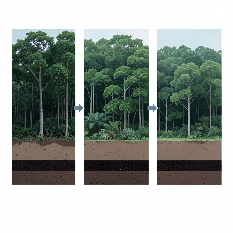
Forest Area and Carbon Correlation
AI-generated conceptual illustration (Subtropical forests in Banke, Nepal). It explains the idea and does not show study data.
View source evidence ↗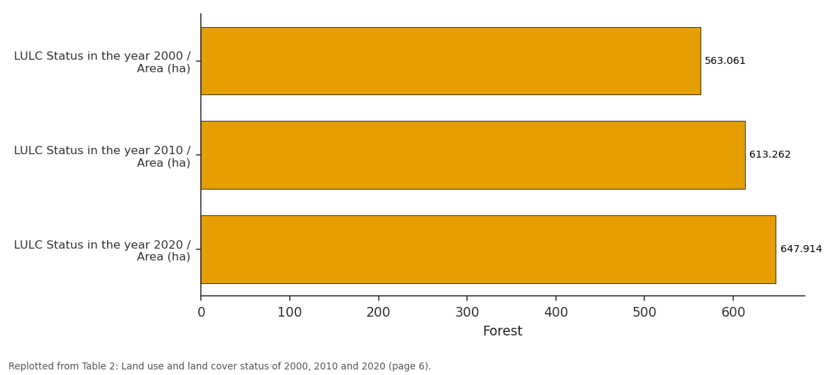
Forest: LULC Status in the year... vs LULC Status in the year... vs LULC Status in the year...
Replotted from Table 2 (page 6) of the original paper. Every bar is the paper's own table value.
View source evidence ↗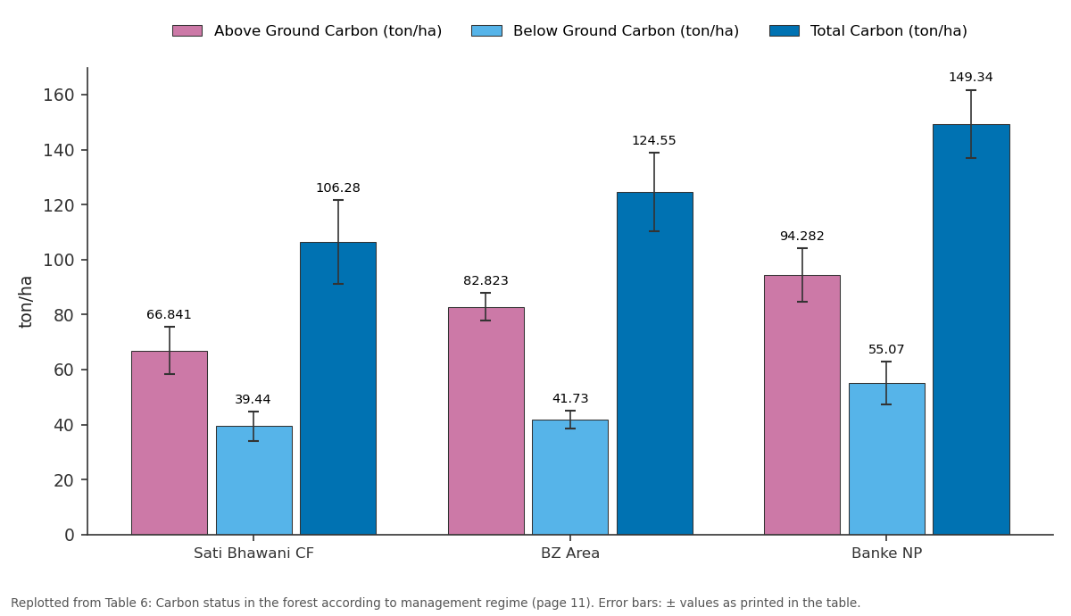
Above Ground Carbon (ton/ha) and Below Ground Carbon (ton/ha) and more: Sati Bhawani CF vs BZ Area vs Banke NP
Replotted from Table 6 (page 11) of the original paper. Every bar is the paper's own table value.
View source evidence ↗Figures & tables
From the original paper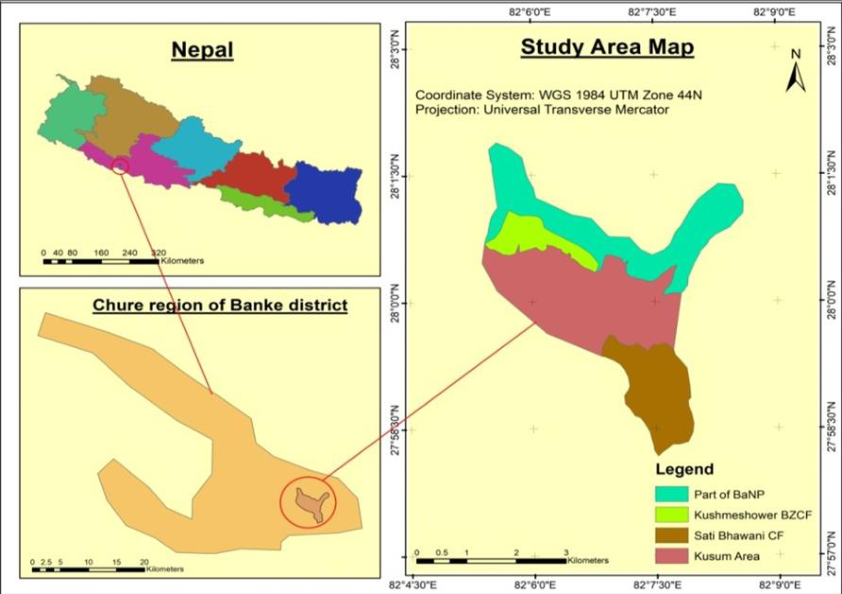 Figure 1
 Table 1
 Table 2
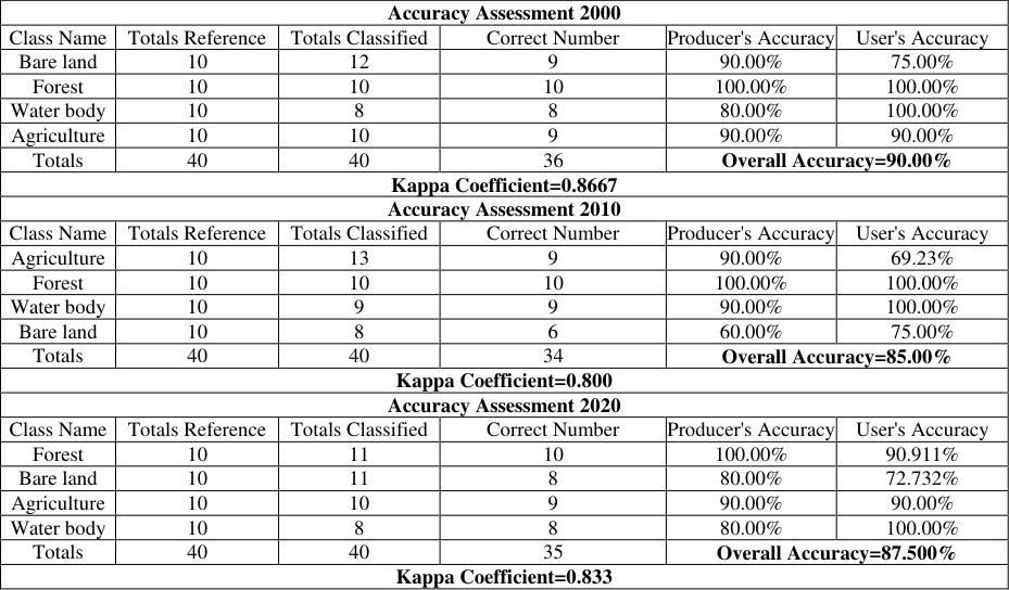 Table 3
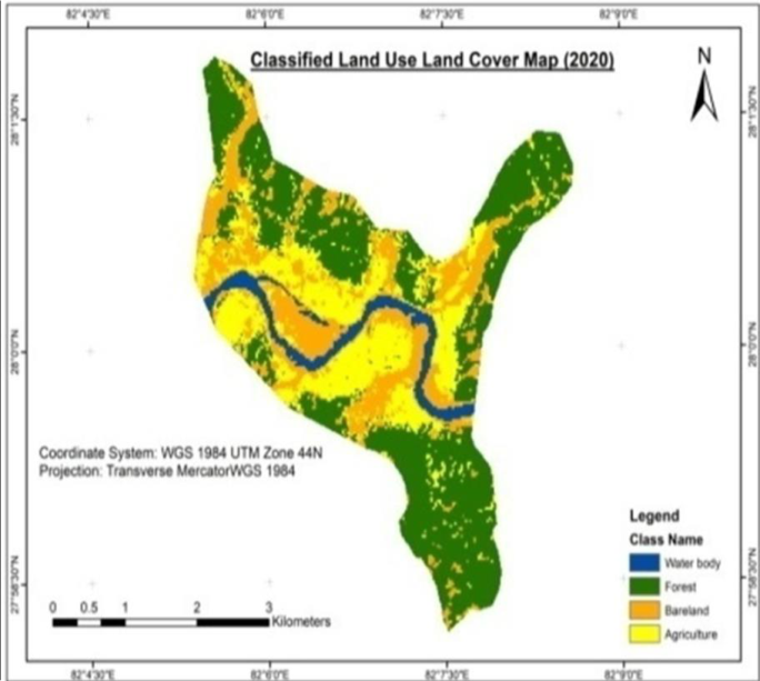 Figure 2
 Table 4
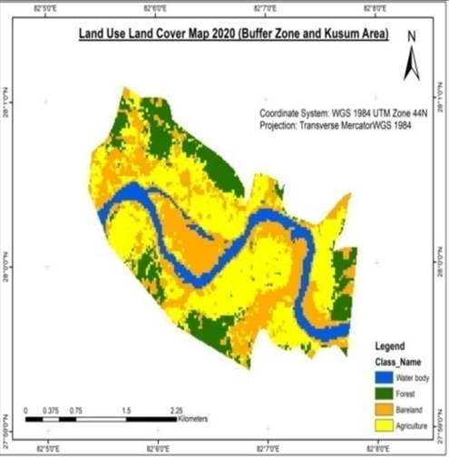 Figure 3
 Table 5
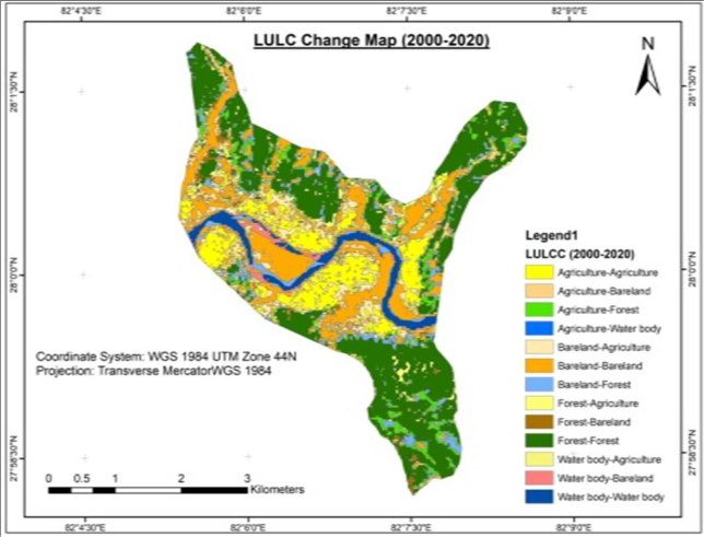 Figure 4
 Table 5
 Table 5
 Table 6
 Table 7
 Table 8
Introduction
The change in land use land cover is the indicator of deforestation which affects the forest carbon but it is difficult to monitor. The remote sensing techniques using the change detection shows change in land use and land cover and their effect on carbon stock. Changes in land cover have a direct effect on carbon sequestration in vegetation cover with an influence on climate on a continental scale (Schulp et al., 2008, Sharma & Kakchapati, 2018) [27, 28] . There are several researches regarding this to evaluate the carbon stock change using different types of remote sensing techniques. Global deforestation is challenging one and the remote sensing techniques are used to assess and monitor the carbon stock. Even, the remote sensing techniques are used to assess the forest degradation as well. Land cover has a direct effect on Carbon stock (Mahmod et al.,2010, Ishtiaque et al., 2017, Mauya et al., 2019) [17,22] . The deforestation and forest degradation affect the carbon stock in the forests (Ray et al., 2011, Ghimire, 2017) [25,13] . Tropical deforestation is alarming and consequence is lowering the carbon stock. India, Bhutan, Pakistan and Sri Lanka are facing the serious problem of deforestation and forest degradation and so as Nepal. Chure range is distributed from low hill from Indus River in Pakistan in the west throughout the length of Nepal until it reaches Bramhaputra River in India in the east. The Chure-Terai Madhesh landscape region is ecologically diverse and so carbon stock is also diverse. This region is environmentally degraded and structurally weak and fragile due to deforestation, forestland fragmentation and encroachment, rural road construction, overgrazing, forest fire, cultivation on the steep slopes, and soil erosion (Editor., 2015) [9] . Terai region geographically consists of Chure, Bhabar, and Plain areas of Nepal (Acharya et al., 2019) [1] which is one of the country's most fragile landscape with friable soils, high vulnerability to various natural hazards such as extreme heat, water scarcity, wildfires, flooding, and landslides (DFRS, 2014) [7] . The researched are limited in Nepal particularly in Chure areas of Banke district. The existing practice of unmanaged cultivation, deforestation, improper use of agrochemicals, unmanaged and unscientific construction of roads, buildings, and excessive sand and stone quarrying are some of the anthropogenic activities leading to soil erosion and landslides, which ultimately influence negatively on forest carbon. The studies on land use land cover change generally been conducted in different areas but specifically research on the effect of land use land cover change on forest carbon was a major gap. After the establishment of Banke National park, the study regarding the Chure area is less. Realizing this gap, the current study is felt to be very important. Thus, this research was objectively conducted to assess the effects of land use and land cover changes on forest carbon in community forest, buffer zone community forest and national park in Chure area of Banke district, Nepal.
Materials and Methods
Study Area: The Chure area of Banke district is situated between 81°39'29" to 82°12'19"E latitude and 27°58'13" to 28°21'23"N longitude in the Terai region, a part of Province No. 5 in the mid-western part of our country Nepal. Chure covers the area 37.8% of Banke district which is also the part of Banke national park with three climatic zones namely Lower Tropical with elevation range below 300m covering an area of 79.1%, Upper Tropical climatic Zones with elevation range 300-1000m covering an area of 20.6% and Sub-Tropical with elevation range 1000-2000m covering an area of 0.3%. Chure hills are rugged, which are deeply dissected by gullies and streams. Escarpments and ant-dip steep slopes are common slope features as evidence of geological control and erosion. Chure hill slopes are generally dry and have poor soil development. Within the Chure range there exist several notable inner river valleys comprising small flood plains and river terraces of two or three tiers at some east-west sections. Average Temperature ranges between 39 °C to 6°C whereas average rainfall is around 1362mm. Total area of the Banke district is 233700 ha in which 80871.1 ha area is covered by the Chure area. According to the report presented by division forest office Banke, forest land cover about 132959 ha, Agriculture land covers about 92068 ha, Shrubs land covers about 5375 ha, barren land covers about 2337 ha and other land covers about 931 ha. There is about 119939.74 ha forest area in Banke district. Out of this, 62200.68 ha (51.86%) is under Banke National Park and remaining 57739.06 ha (48.14%) is under National Forest. Similarly, there are 119 Community Forests (CFs) and 53 Buffer Zone Community Forest (BZCF). According to Land Resource Mapping Project, Chure Forest is divided into three types as Hardwood, Mixed forest, and Shrubs. Mainly Sal (Shorea robusta) (Tropical Mixed Hardwood/Sal) is the main Species in Banke District whereas Khayer (Acacia Catechu), Sissoo (Dalbergia sissoo) are the species found near the river. Major non timber forest species includes Kurilo (Asparagus racemosus), Bel (Aegal marmelos), Barro (Terminalia bellerica), Harro (Termenalia chebula), Amala (Phylanthus emblica), Simal (Bombax ceiba) etc. (DFRS, 2014) [6] . The Chure area of the Banke district holds major wild-life animal species such as Tiger (Panthera tigris), four-horned antelope (Tetracerus quadricornis) etc. The study sites are Rapti Sonari Rural Municipality situated in the Chure region of Banke district which is around 500 km from Kathmandu valley. Eastern part of Kusum Area, Sati Bhawani Community Forest, Kusmeshower Buffer Zone Community Forest, and part of Banke National Park have been selected for the research study through consultation with President Chure Terai Madhesh Conservation Development Board and Division Forest Office (DFO) (figure 1).
Research design
Data Collection: Primary and secondary data were collected. In addition to these spatial data was also collected to analyze the effect of LULC on forest carbon. Primary data were collected from field observation, direct measurement, key Informant Interviews, laboratory analysis while the secondary data and information were collected from internet surfing, books, reports, journals, and community forest operational plans to meet the research objectives. Two Landsat 7 ETM+ and one Landsat 8 OLI/TIRS Satellite images dated 2000, 2010 and 2020 were used to find a change between these periods. Both satellite images were downloaded from the United States Geological Survey (USGS) official website (https://earthexplorer.usgs.gov/) (Table 1) Priority was given to the data with less cloud cover and sensor noise, and at the same time attention was made for acquiring images with smaller seasonal variations.
Aboveground and below ground biomass:
The diameter at breast height (DBH) at 1.3m height and height of individual tree greater than 10cm DBH were measured within 8.92 m radius using diameter tape, starting from the edge and working inwards, marking each tree as to prevent accidental double counting. Meanwhile, the height of the trees was measured using Criterion. Sub-plots having a 5.64 m radius inside the tree plots were established for saplings height, diameter and weight measurement. Smaller nested subplots having 1 m radius inside the plots were established for regeneration. Total no of sapling and seedling from these sub-plots were weighed and measured. Smaller nested subplots having 0.56 m radius inside the plots were established and LHG inside the sub-plot were collected, weighed and measured. The soil samples from different places at depth 0-10 cm, 10-20 cm, and 20-30 cm were collected in the soil core sampler of known volume and placed in the labeled sample bag. The collected samples were brought to the laboratory to determine the carbon content. Fresh Weight was taken to measure the bulk density. The soil samples were oven air-dried at air temperature in the laboratory to estimate the soil organic carbon content. [30] . The study area was classified into the 4 LULC classes (Forest, Agriculture, Water Body, and Bare land).
Change analysis:
The classified images were imported in ArcMap 10.2.1 and the area of each class was computed using the "Zonal geometry as Table " tool in Spatial Analyst Extension. Also, the LULC conversion table (Table showing the quantity of one LULC converted into other over three periods) was computed using the "Tabulate Area" tool in Spatial Analyst Extension.
Rate of change in land use and land cover
The following formula was used to compute the rate of change of land cover and land use in the study area.
Rate of change (%) = [(a2/a1)1 /n -1] × 100 (FAO, 1995) [11] Where, a1 = base year data a2 = End year data n = no. of years Accuracy Assessment: An accuracy assessment was carried out using the kappa coefficient. The percentage of agreement gained after eliminating the percentage of agreement that could occur by chance is the kappa coefficient; it lies on a scale between 0 and 1 where 1 represents a complete agreement. Kappa statistic was computed as;
K=N r i=1Xii-r i=1 (Xi*Xx+1)/N 2 -r i=1 (Xi*Xx+1) (Cohen, 1995) [5] Where; r = number of rows and columns in error matrix, N = total number of observations (pixels) Xii = observation in row i and column i, Xx+i = marginal total of row i, and Xx+i = marginal total of column i Aboveground Tree/Pole/Sapling Biomass Calculation: AGTB = 0.0509 x ρD 2 H (Chave et al., 2005) [4] .
Whereas, AGTB = above ground tree biomass (kg) ρ = dry wood density (gm/cm 3 ) D = tree diameter at breast height (cm) H = tree height (m) After taking the sum of all the individual weights in kg of a sampling plot and dividing it by the area of a sampling plot (m 2 ), the tree biomass stock was attained in kg/m 2 . This value was converted to t/ha by using the unitary method. Above ground sapling/Seedling biomass calculation: To determine the aboveground sapling/seedling biomass fresh weight was taken from the sample plots. Litter, Herbs and Grass Biomass (LHGB) calculation: LHG = (W field /A) × (W sample, dry/W sample, wet) × 1/10000 Where, LHG= Biomass of leaf litter, herbs, and grass (t/ha) W field = weight of the fresh field sample of leaf litter, herbs, and grasses, which was sampled destructively within the given area in (g) A = size of the area in which leaf litter, herbs, and the grass was collected (ha); W sample, dry = weight of the oven-dry sub-sample of leaf litter, herbs and grasses that was taken to determine moisture content (g); (Approximately 40% of the fresh weight) And W sample, wet = weight of the fresh sub-sample of leaf litter, herbs, and grasses that was taken to determine moisture content (g) Below ground tree/pole carbon stock: Below ground biomass was estimated as 25% of aboveground tree/pole biomass (Mac Dicken, 1997) [20] .
Soil organic carbon:
The soil samples were analyzed by Walkley Black Method (Walkley & Black, 1958) [33] by digestion using Sulphuric acid and oxidized by the Potassium dichromate in the laboratory. The soil samples were oven-dried at room temperature in the laboratory for 3 days to remove moisture from the sample. The bulk density of the soil sample was calculated for each soil depth for which soil carbon was estimated. Then, ovendried soil samples were divided by its volume to estimate bulk density. For the calculation of soil organic carbon (SOC), the following formula was used (Chabbra et. al, 2002). Bulk Density (gm/cm 3 ) = (oven-dry weight of soil) / (volume of soil in the core). SOC= Organic Carbon Content % * Soil Bulk Density (gm/cm 3 )*thickens of the horizon and was expressed in tons per ha. Whereas, SOC = soil organic carbon stock per unit area (t/ha), % C = carbon concentration ρ = soil bulk density (gm/cm 3 ) & d = total depth at which the sample was taken (cm) Default value i.e. root shoot ratio 0.125 was used (IPCC, 2006) to calculate the root biomass. The root shoot ratio of 0.125 was multiplied in the above-ground biomass for the biomass of root. Similarly, the universal conversion factor generally, 0.47 was used to convert dry biomass of tree, pole, sapling, regeneration, herbs, litter, grasses, and dead wood into carbon content (Andreae & Merlet, 2001) [2] .
Estimation of forest carbon based on business as usual scenario
The present carbon stock is estimated based on the field data of 2020. The image classification of 2000 revealed that 39.40 percent of total land was covered by forest which was the major land cover type in the study area, whereas Agriculture occupying 23.78 percent was the major land use. Bare land and water occupied 31.30 percent and 5.50 percent respectively. Similarly, the image classification of 2010 showed that forest remains the major land cover type covering 42.92 percent of total land. Similarly, Agriculture is still the major land use occupying 16.34 percent. Bare land and water cover 34.52 percent and 6.20 percent respectively; in the year 2020 also Forest remains the major land cover occupying 45.34 percentages whereas Agriculture remains the major land use occupying 24.45 percentages. Bare land and water occupied 24.91 percent and 5.28 percent respectively (Table 2, figure 2). 3). The Accuracy was 90% of the classified map of 2000, 85% of 2010 and 87.55% of 2020. The figure and table depict that the highest amount of land cover change had taken place from Agriculture land to bare land (9.49%), Agriculture to forest (5.64%), and from forest to bare land (5.78%) in the period between 2000 and 2010. Similarly, a small amount of conversion had taken place from bare land to water body and all other's conversion is below 1% hence neglected. The highest amount of land cover change had taken place from Agriculture land to bare land (10.72%) and forest to bare land (7.42%) in the period between 2010 and 2020.
| SN | LULC Classes | LULC Status in the year 2000 | — | LULC Status in the year 2010 | — | LULC Status in the year 2020 | — |
|---|---|---|---|---|---|---|---|
| Area (ha) | Area (%) | Area (ha) | Area (%) | Area (ha) | Area (%) | ||
| 1 | Forest | 563.061 | 39.400 | 613.262 | 42.921 | 647.914 | 45.341 |
| 2 | Agriculture | 339.812 | 23.781 | 233.543 | 16.343 | 349.401 | 24.452 |
| 3 | Bare land | 447.261 | 31.302 | 493.314 | 34.522 | 355.982 | 24.911 |
| 4 | Water body | 78.541 | 5.501 | 88.581 | 6.204 | 75.501 | 5.281 |
| Grand Total | 1429 | 100 | 1429 | 100 | 1429 | 100 |
Table text extracted from the original PDF; superscript letters are shown inline. The original table image is below.
View original table image
Similarly, a small amount of conversion had taken place from Agriculture to forest, bare land to forest and bare land to water body whereas all other's conversion is below 1% hence neglected. Also, the figure and table shows that the highest amount of land cover change had taken place from bare land to Agriculture (8.05%), Agriculture land to the forest (5.84%), and Agriculture to bare land (5.12%) in the period between 2000 and 2020. Similarly, a small amount of conversion had taken place from bare land to forest and Forest to Agriculture whereas all other conversions are below 2% hence neglected (Figure 4, Table 5). was decreased from 2000 to 2010 that was -3.68% but and it was increased by 4.11% from 2010 to 2020 (Table 5). In the Nepalese forest, an average carbon stock account to 203 t ha -1 (including shrub land) which is higher than the world's average i.e. 161.1 t ha -1 (FAO, 2006) [11] . In this study, the average carbon stock of three community forests [12] . Also from the report present by the DFRS (2015) [6] in the whole country, the forest area was increased from 39.6% to 44.74%. Similarly, one of the major changes in land use is Agriculture land which was decreased by 6.56% from 2000 to 2010 and it was again increased by 7.23% from 2010 to 2000 the reason behind the change in Agriculture land is urbanization. Most of the villagers either migrated towards the city or choose any other profession for livelihood in recent years. This reason was also supported by the author Paudel et al., (2017) [24] . People's perception is one of the [3] . Total carbon stock was found to be highest in Banke national park in Chure region with 149.34 ton/ha which was because of presence of dense forest. The National park was applying the conservation practices which lead to restrict the removal of logging and encroachment. Another important part is application of buffer zone community forest management and community forest management which emphasize to reduce the logging and encroachment. Various author Khadka et al., (2019) [19] concluded that forest under the protected areas of Nepal had higher amount of total carbon stock per hectare compared to the forest outside the protected area. Similarly, Sapling and seedling carbon stock was found to be highest in Community forest i.e. 2.08 ton/ha which was due to the scientific management practices applied in Community forest which results to increase in the regeneration forest. The soil carbon stock was found to be highest in the National Park of Chure region with 43.287±5.658t C ha -1 . Land use and soil depth both affected the SOC (Ghimire et al., 2019) [35] . The clear trend was seen in soil carbon according to the soil depth. It was highest in 0-10 cm while lowest in 20-30 cm depth which was supported by the author Sah et al., (2019) [26] . The soil carbon was highest in the upper layer and it decreases according to the soil depth due to rapid decomposition of forest litter in a upper layer (Mandal et al., 2019) [19] . When time changes forest area also changes mainly there was degradation and the deforestation of the forest area. Change in forest area can be measured easily but it is difficult to measure the effect of land use land cover change in the forest area which needs high quality data. So, we use usual scenario to find effect of land use land cover change on forest carbon of the year 2000 and 2010.
| LULC Classes | Rate of Increment(%) and Decrement(-%) per Year | — |
|---|---|---|
| From 2000 to 2010 | From 2010 to 2020 | |
| Forest | 0.861 | 0.550 |
| Agriculture | -3.682 | 4.110 |
| Bare Land | 0.981 | -3.210 |
| Water body | 1.214 | -1.580 |
Table text extracted from the original PDF; superscript letters are shown inline. The original table image is below.
View original table image
| — | Forest(ha) | 4.019 | 106.082 | 538.88 | 0.362 | 649.344 |
|---|---|---|---|---|---|---|
| Water body(ha) | 1.541 | 9.181 | 1.126 | 63.560 | 75.411 | |
| Grand Total(2010) (ha) | 232.911 | 493.312 | 614.035 | 88.450 | 1429 | |
| Change between 2000 & 2020 | LULC Change | Agriculture | Bare land | Forest | Water body | Grand Total(2000) |
| Agriculture(ha) | 185.503 | 73.127 | 83.448 | 0.189 | 342.268 | |
| Bare land(ha) | 114.991 | 249.116 | 66.328 | 16.352 | 446.786 | |
| Forest(ha) | 46.011 | 18.983 | 496.919 | 0 | 561.914 | |
| Water body(ha) | 2.280 | 17.326 | 0 | 58.908 | 78.515 | |
| Grand Total(2020) (ha) | 348.785 | 358.554 | 646.695 | 75.450 | 1429 |
Table text extracted from the original PDF; superscript letters are shown inline. The original table image is below.
View original table image
| Change between 2000 & 2010 | LULC Change | Agriculture | Bare land | Forest | Water body | Grand Total(2000) |
|---|---|---|---|---|---|---|
| Agriculture(ha) | 122.791 | 135.631 | 80.711 | 1.171 | 339.812 | |
| Bare land(ha) | 105.452 | 264.462 | 55.512 | 21.842 | 447.263 | |
| Forest(ha) | 4.231 | 82.696 | 475.844 | 0.293 | 563.054 | |
| Water body(ha) | 1.563 | 10.531 | 1.195 | 65.266 | 78.545 | |
| Grand Total(2010)(ha) | 233.541 | 493.312 | 613.261 | 88.554 | 1429 | |
| Change between 2010 & 2020 | LULC Change | Agriculture | Bare land | Forest | Water body | Grand Total (2020) |
| Agriculture(ha) | 150.629 | 153.164 | 41.005 | 2.642 | 347.441 | |
| Bare land(ha) | 76.721 | 224.885 | 33.022 | 21.884 | 356.513 |
Table text extracted from the original PDF; superscript letters are shown inline. The original table image is below.
View original table image
Business as usual scenario total carbon stock of 2020 was 82103.16 ton. Various author Sharma and Rai, (2007) [29] explained that land use land cover change have direct effect on the forest carbon so, from assumption, we found total carbon of 2000 was 71350.96 ton in which when forest area decreases carbon stock also decreases. LULCC have direct effect on the Carbon stock but Land-cover did not significantly affect SOC concentrations in non-domestic green space, but values beneath trees were higher than under both pasture and arable land, whereas concentrations under shrub and herbaceous land-covers were only higher than arable fields (Edmondson et al., 2015) [8] . The sources and sinks of carbon from LULCC are significant in the global carbon budget. Deforestation and other land-cover changes are responsible for 53-58% of the difference between current and potential biomass stocks (Erb et al., 2018). Thus, land use change effects and forest carbon cycling during different period are dominated by changes in tree carbon stocks (Woodbury et al., 2006). So in overall comparison when the land cover on the given area was decreased carbon stock also decreased.
Conclusion and Recommendations
The land use land cover change map showed that forest area was less in 2000 which was increased in 2010 and the increase was continued to 2020 as well. The above ground tree/pole carbon stock was found to be highest in National Park of Chure region because of dense forest but the forest carbon was the lowest in community forest. Similar result was found that the soil carbon was found to be highest in National Park of Chure region. The carbon stock was increasing from 2000 to 2020 since the forest area was increased in this period. Assuming 10% less carbon in 2000 and 2010, the total forest carbon of 2010 and 2000 would be less and hence total CO2 equivalent would also be less and same principle is applied for assuming other scenario. Effect of land use and land cover change was monitored using remote sensing analysis which can be useful tool for forest manager and policy maker. The carbon stock in Chure forest managed under the national park can be used as reference for other part of Nepal as well. The increasing trend of carbon and their link with the land use land cover change will be useful to develop the policy related to carbon enhancement. Carbon assessment study should be extended to all over Chure area of Nepal and this should be linked with the land use land cover change.
Figures and tables from the paper
| Accuracy Assessment 2000 | — | — | — | — | — |
|---|---|---|---|---|---|
| Class Name | Totals Reference | Totals Classified | Correct Number | Producer's Accuracy | User's Accuracy |
| Bare land | 10 | 12 | 9 | 90.00% | 75.00% |
| Forest | 10 | 10 | 10 | 100.00% | 100.00% |
| Water body | 10 | 8 | 8 | 80.00% | 100.00% |
| Agriculture | 10 | 10 | 9 | 90.00% | 90.00% |
| Totals | 40 | 40 | 36 | Overall Accuracy=90.00% | |
| Kappa Coefficient=0.8667 | |||||
| Accuracy Assessment 2010 | |||||
| Class Name | Totals Reference | Totals Classified | Correct Number | Producer's Accuracy | User's Accuracy |
| Agriculture | 10 | 13 | 9 | 90.00% | 69.23% |
| Forest | 10 | 10 | 10 | 100.00% | 100.00% |
| Water body | 10 | 9 | 9 | 90.00% | 100.00% |
| Bare land | 10 | 8 | 6 | 60.00% | 75.00% |
| Totals | 40 | 40 | 34 | Overall Accuracy=85.00% | |
| Kappa Coefficient=0.800 | |||||
| Accuracy Assessment 2020 | |||||
| Class Name | Totals Reference | Totals Classified | Correct Number | Producer's Accuracy | User's Accuracy |
| Forest | 10 | 11 | 10 | 100.00% | 90.911% |
| Bare land | 10 | 11 | 8 | 80.00% | 72.732% |
| Agriculture | 10 | 10 | 9 | 90.00% | 90.00% |
| Water body | 10 | 8 | 8 | 80.00% | 100.00% |
| Totals | 40 | 40 | 35 | Overall Accuracy=87.500% | |
| Kappa Coefficient=0.833 |
Table text extracted from the original PDF; superscript letters are shown inline. The original table image is below.
View original table image
| LULC | Banke National Park: | — | — | Sati-Bhawani Community Forest | — | — | Buffer Zone Area | — | — |
|---|---|---|---|---|---|---|---|---|---|
| 2000 | 2010 | 2020 | 2000 | 2010 | 2020 | 2000 | 2010 | 2020 | |
| Forest (ha) | 274.09 | 288.72 | 339.01 | 197.83 | 244.88 | 236.42 | 108.99 | 104.01 | 119.16 |
| Bare Land (ha) | 170.29 | 155.82 | 105.45 | 35.113 | 21.364 | 24.662 | 298.35 | 310.33 | 241.11 |
| Water Body (ha) | 0.057 | 0.017 | 0.067 | 0 | 0 | 0 | 80.485 | 89.502 | 75.222 |
| Agriculture (ha) | 0 | 0 | 0 | 36.699 | 3.822 | 9.280 | 226.657 | 210.533 | 278.295 |
| Total (ha) | 445 | 445 | 445 | 270 | 270 | 270 | 714 | 714 | 714 |
Table text extracted from the original PDF; superscript letters are shown inline. The original table image is below.
View original table image
| — | Above Ground Carbon (ton/ha) | Below Ground Carbon (ton/ha) | Total Carbon (ton/ha) |
|---|---|---|---|
| Sati Bhawani CF | 66.841±8.621 | 39.44±5.324 | 106.28±15.285 |
| BZ Area | 82.823±5.101 | 41.73±3.241 | 124.55±14.231 |
| Banke NP | 94.282±9.689 | 55.07±7.820 | 149.34±12.386 |
Table text extracted from the original PDF; superscript letters are shown inline. The original table image is below.
View original table image
| — | Data type | Type of test | P-value | Decision |
|---|---|---|---|---|
| Tree/Pole | Not normal | Kurskal wallis | 0.111 | Not significant |
| Sapling | Normal | One Way ANOVA | 0.001 | Significant |
| Seedling | Not normal | Kurskal wallis | 0.001 | Significant |
| LHG | Normal | One Way ANOVA | 0.290 | Not Significant |
| Soil Carbon | Normal | One Way ANOVA | 0.051 | Not Significant |
Table text extracted from the original PDF; superscript letters are shown inline. The original table image is below.
View original table image
References
35 in the original paper- Acharya RP, Maraseni TN, Cockfield G. Local Users and Other Stakeholders' Perceptions of the Identification and Prioritization of Ecosystem Services in Fragile Mountains: A Case Study of Chure Region of Nepal. Forests 2019;10(5):421. https://doi.org/10.3390/f10050421
- Andreae, Merlet. "Emission of trace gases and aerosols from biomass burning", global biogeochemical cycles, 2001;15(4):955-966.
- Chaudhari PR, Ahire DV, Ahire VD, Chkravarty M, Maity S. Soil Bulk Density as related to Soil Texture, Organic Matter Content and available total Nutrients of 2013;3:1-8.
- Chave J, Andalo C, Brown C. "Tree allometry and improved estimation of carbon stocks and balance in tropical forests", Oecologia 2005;145:87-99.
- Cohen J. A coefficient of agreement for nominal scales. Educational and psychological measurement 1960;20(1):37-46.
- FRA/DFRS. Churia Forests of Nepal (2011 -2013). Babarmahal, Kathmandu: Forest Resource Assessment Nepal Project/Department of Forest Research and Survey, 2014.
- DFRS. "Community forestry Inventory Guideline 2003" Department of Forest Research and Survey, Babarmahal, Kathmandu, Nepal, 2003.
- Edmondson JL, Davies ZG, McCormack SA, Gaston KJ, Leake JR. Land-cover effects on soil organic carbon stocks in a European city. Science of The Total Environment 2014;472:444-453. https://doi.org/10.1016/j.scitotenv.2013.11.025
- Editor T. Chure Conservation: Efforts and Challenges in Nepal. Banko Janakari 2015;24(1):1-2. https://doi.org/10.3126/banko.v24i1.13472
- Erb KH, Kastner T, Plutzar C, Bais ALS, Carvalhais N, Fetzel T et al. Unexpectedly large impact of forest management and grazing on global vegetation biomass. Nature 2018;553(7686):73-76. https://doi.org/10.1038/nature25138
- FAO. 1995. Forest resources assessment 1990. Global Synthesis. FAO, Rome. Retrieved from http://www.fao.org/docrep/007/v5695e/v5695e00.htm
- Gautam AP, Webb EL, Eiumnoh A. GIS Assessment of Land Use/Land Cover Changes Associated With Community Forestry Implementation in the Middle Hills of Nepal. Mountain Research and Development, 2002;22(1):63-69. https://doi.org/10.1659/02764741(2002)022[0063:GAOLUL]2.0.CO;2
- Ghimire M. Historical Land Covers Change in the Chure-Tarai Landscape in the Last Six Decades: Drivers and Environmental Consequences. In A. Li, W. Deng, & W. Zhao (Eds.), Land Cover Change and Its Eco-environmental Responses in Nepal 2017, 109-147.
- Islam M, Kader MA, Md. Bhuiyan SH, Chowhan S, Talukder JA, Md. Rahman M, et al. Effect of long term fertilization on soil respiration and enzyme activities in floodplain soil. Int. J Res. Agron. 2019;2(2):29-34. DOI: 10.33545/2618060X.2019.v2.i2a.20
- He JF, Liu JY, Zhuang DF, Zhang W, Lu ML. Assessing the effect of land use/land cover change on the change of urban heat island intensity. Theoretical and Applied Climatology 2007;90(3):217-226. https://doi.org/10.1007/s00704-006-0273-1
- IPCC. "IPCC Guidelines for National Greenhouse Gas Inventories". National Greenhouse Gas Inventories Programme, Eggleston HS, Buendia L, Miwa K, Ngara T, Tanabe K. (eds). Published: IGES, Japan. 2006.
- Ishtiaque A, Shrestha M, Chhetri N. Rapid Urban Growth in the Kathmandu Valley, Nepal: Monitoring Land Use Land Cover Dynamics of a Himalayan City with Landsat Imageries. Environments 2017;4(4):72. https://doi.org/10.3390/environments4040072
- Jiang J, Tian G. Analysis of the impact of Land use/Land cover change on Land Surface Temperature with Remote Sensing. Procedia Environmental Sciences 2010;2:571-575. https://doi.org/10.1016/j.proenv.2010.10.062
- Khadka G, Mandal R, Mathema A. Comparison Growing Stock, Carbon Stock and Biodiversity in and Around Banke National Park, Nepal. International Journal of Botany 2019;5:21-26.. https://doi.org/10.20431/2455-4316.0503004
- Mac Dicken KG. A Guide to Monitoring Carbon Storage in Forestry and Agroforestry Projects, 1997, 91.
- Mandal RA, Dutta IC, Jha PK, Karmacharya SB. Carbon sequestration potential in community and collaborative forests in Terai, Nepal, 2016. /paper/Carbon-sequestration-potential-in-communityand-in-MandalDutta/082675ee04036398ff8518117b712412324b3515
- Mauya E, Mugasha W, Njana M, Zahabu E, Malimbwi RE. Carbon stocks for different land cover types in Mainland Tanzania. Carbon Balance and Management, 2019;14:4. https://doi.org/10.1186/s13021-019-0120-1
- Mahmood et al. Impacts of Land UseLand Cover Change on Climate a.pdf. (n.d.). Retrieved, 2020, from https://journals.ametsoc.org/doi/pdf/10.1175/2009BAM S2769.1
- Paudel B, Zhang Y, Li S, Wu X. Spatiotemporal reconstruction of agricultural land cover in Nepal from 1970 to 2010 Regional Environmental Change 2017;17(8):2349-2357. https://doi.org/10.1007/s10113017-1164-y
- Ray R, Ganguly D, Chowdhury C, Dey M, Das S, Dutta MK et al. Carbon sequestration and annual increase of carbon stock in a mangrove forest. Atmospheric Environment 2011;45(28):5016-5024. https://doi.org/10.1016/j.atmosenv.2011.04.074
- Sah S, Sharma S, Mandal R. Comparison of Carbon Stock in Chure, Bhawar and Terai, Nepal (A study from Mahottary district). International Journal of Scientific and Engineering Research 2019;10:80-93.
- Schulp CJE, Nabuurs GJ, Verburg PH. Future carbon sequestration in Europe-Effects of land use change. Agriculture, Ecosystems & Environment 2008;127(3):251-264. https://doi.org/10.1016/j.agee.2008.04.010
- Sharma I, Kakchapati S. Linear Regression Model to Identify the Factors Associated with Carbon Stock in Chure Forest of Nepal [Research Article]. Scientifica 2018. https://doi.org/10.1155/2018/1383482
- Sharma P, Rai SC. Carbon sequestration with land-use cover change in a Himalayan watershed. Geoderma 2007;139(3):371-378. https://doi.org/10.1016/j.geoderma.2007.02.016
- Sisodia PS, Tiwari V, Kumar A. Analysis of Supervised Maximum Likelihood Classification for remote sensing image. International Conference on Recent Advances and Innovations in Engineering (ICRAIE-2014), 2014, 1-4. https://doi.org/10.1109/ICRAIE.2014.6909319
- Turner B, Skole D, Sanderson S, Fischer G, Fresco L, Leemans R. Land-Use and Land-Cover Change: Science/research plan, 1995. [No Source Information Available]. https://asu.pure.elsevier.com/en/publications/land-useand-land-cover-change-scienceresearch-plan-2
- Verburg PH, van Eck JRR, de Nijs TCM, Dijst MJ, Schot P. Determinants of Land-Use Change Patterns in the Netherlands. Environment and Planning B: Planning and Design 2004;31(1):125-150. https://doi.org/10.1068/b307
- Walkley AE, Black JA. "An Examination of the Degtjareff Method for Determining Soil Organic Method, and Proposed Modification of the Chromic Acid Titration Method" 1958;37:29-38.
- Woodbury PB, Heath LS, Smith JE. Land Use Change Effects on Forest Carbon Cycling Throughout the Southern United States. Journal of Environmental Quality 2006;35(4):1348-1363. https://doi.org/10.2134/jeq2005.0148.
- Ghimire Pramod, Bhatta B, Pokhrel B, Kafle G, Paudel P. Soil organic carbon stocks under different land uses in Chure region of Makawanpur district, Nepal. SAARC Journal of Agriculture 2019;16:13-23. https://doi.org/10.3329/sja.v16i2.40255
Cited by 1
From OpenAlex, OpenCitations and reference lists read by Scinovex
- Forest Structure, Diversity, and Regeneration in a Community‐Managed Forest of Nepal: A Model for Carbon Sequestration and Sustainable Management ↗
Tika Ram Poudel, Prakash Chandra Aryal, Muhammad Tayyab Khan, Nathan James Roberts, Manasi Poudel, Dam Prasad Shrestha · Plant-Environment Interactions · 2025
Community forestry, a participatory forest management system, encourages forest conservation, enhances carbon sequestration, and advances the Sustainable Development Goals (SDGs) by increasing community ownership of resource management. Community forestry, in terms of policies and practices, directly supports SDG-1, SDG-13, and SDG-15 by promoting community ownership and empowerment as well as ecosystem health. It provides immediate benefits to local livelihoods by…
❝ 9PDF
Social
Social