
Research article · 2021 · Full text
International Journal of Geography Geology and EnvironmentRecharging of groundwater by the geophysical method based on resistivity meter, a case study of Naya Raipur Chhattisgarh
Volume 3(2) · Pages 69–77 · DOI: 10.22271/27067483.2021.v3.i2a.61 ↗
Research areasGeophysical and Geoelectrical MethodsWater Systems and OptimizationGroundwater and Watershed Analysis
Abstract
Author-writtenTo maintain the balance in the water table, artificial recharge is being adopted in many regions. For this, numerous studies have been carried out. In the present study, vertical electric soundings have been carried out in the different locations of surrounding Atal Nagar, Naya Raipur at 09 random sites to understand the nature and extent of the aquifer and to find out the groundwater potential zone for rainwater harvesting sites. The main objective of this study is to identify the possibility of an appropriate recharge structure at a suitable location. From the interpretation of the VES curve, the evaluation of layer parameters has been done depicting the actual depth of aquifers and high yielding fracture zones. The VES curve has been made to interpret the subsurface geological layers which indicate the 3 to 4 subsurface layers having different resistivity and thickness. When this VES data is correlated with the lithology data of the area, the actual groundwater bearing zone and potential zone can be identified.
Summary
Source-checkedPlain-language reading of the full paper, prepared with AI and checked against the text. Each point links to the authors' own words.
Why it matters
- Groundwater is a critical global resource, accounting for approximately 20% of the world's fresh water supply and 0.61% of all water. View evidence ↗
- Environmental balance is threatened by the rapid withdrawal of groundwater driven by industrial growth and increasing urban populations. View evidence ↗
- Artificial recharge and rainwater harvesting are identified as the primary methods for restoring depleted groundwater levels. View evidence ↗
The question
- The study aims to determine the feasibility and optimal location for a groundwater recharge structure. View evidence ↗
- The research seeks to understand the aquifer's nature and extent to identify potential groundwater zones for rainwater harvesting in Atal Nagar, Naya Raipur. View evidence ↗
What they did
- The subsurface conditions were analyzed using one Gradient Resistivity Profiling (GRP) and nine Vertical Electrical Soundings (VES). View evidence ↗
- An Aqua meter CRM-50 resistivity meter was employed to conduct the geophysical survey. View evidence ↗
- Sounding utilized both Schlumberger and half Schlumberger configurations, with maximum spreads of 240m for sounding and 200m for profiling. View evidence ↗
- Data regarding apparent resistivity and electrode spacing were interpreted using IPI2WIN software via curve matching. View evidence ↗
What they found
- The weathered formation layer ranges from 9.21 to 11 meters in thickness, with resistivity between 21.7 Ω-m and 33.4 Ω-m. View evidence ↗
- The deepest layer consists of a massive formation characterized by high electrical resistivity, ranging from 883 Ω-m to 973 Ω-m. View evidence ↗
- Factor analysis revealed shallow fractures at depths of 12 to 15 meters and deep fractures at depths of 80 to 85 meters. View evidence ↗
What it means
- The authors conclude that integrating various indicative areas within a GIS environment for groundwater prospect mapping can help resolve water scarcity problems. View evidence ↗
- The authors recommend that further extensive research on groundwater is necessary. View evidence ↗
Visual summary
3 visualsIllustrations explain the paper; charts are replotted from the paper's own table values.
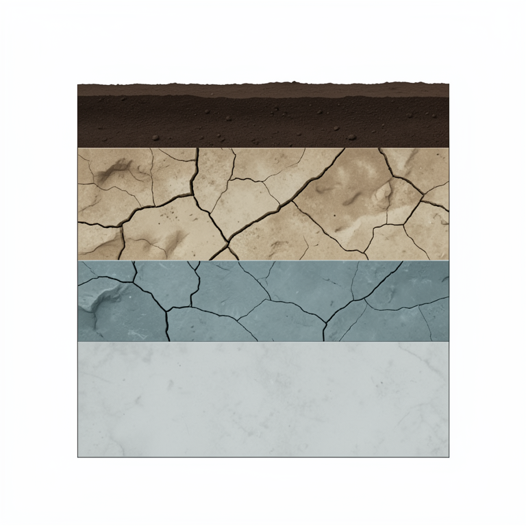
Subsurface Stratigraphy Model
AI-generated conceptual illustration (Subsurface geological stratigraphy of the earth in Naya Raipur, Chhattisgarh). It explains the idea and does not show study data.
View source evidence ↗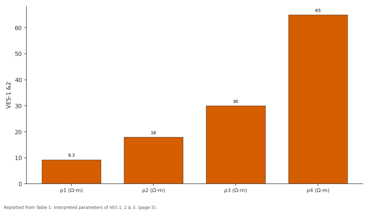
VES-1 &2: ρ1 (Ω-m) vs ρ2 (Ω-m) vs ρ3 (Ω-m) vs ρ4 (Ω-m)
Replotted from Table 1 (page 5) of the original paper. Every bar is the paper's own table value.
View source evidence ↗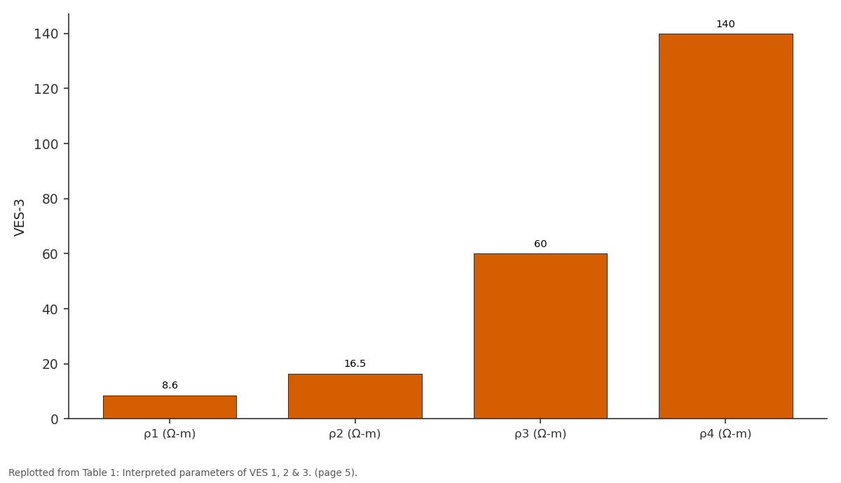
VES-3: ρ1 (Ω-m) vs ρ2 (Ω-m) vs ρ3 (Ω-m) vs ρ4 (Ω-m)
Replotted from Table 1 (page 5) of the original paper. Every bar is the paper's own table value.
View source evidence ↗Figures & tables
From the original paper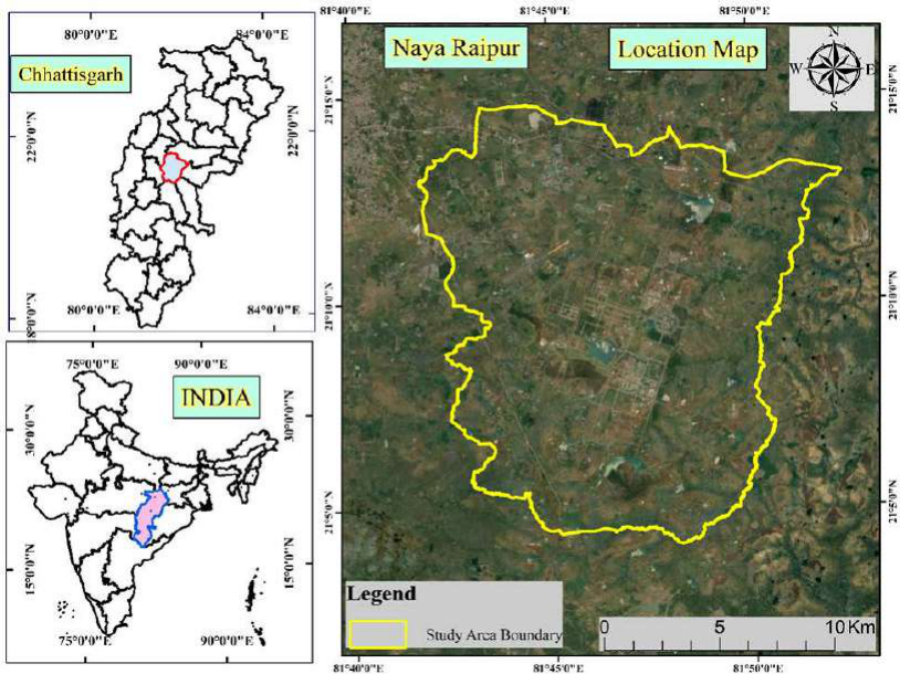 Figure 1
 Table 1
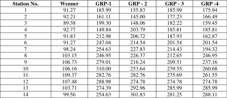 Table 2
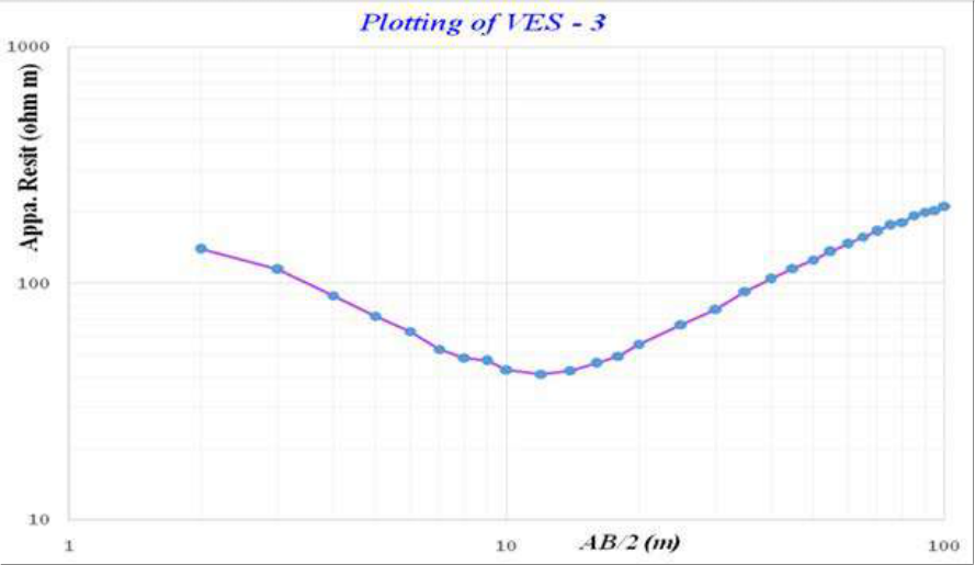 Figure 2
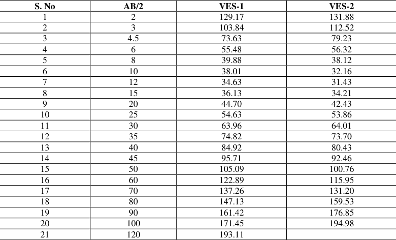 Table 3
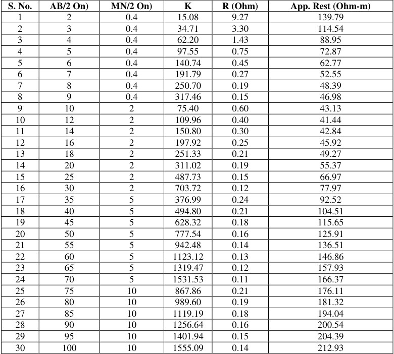 Table 3
Introduction
Water is a vital natural source and life originated in water about 3.2 billion years ago. Twothirds of a living organism consists of water and 90% of cell content is also water. Biochemical reactions in living organisms require an aqueous medium. Therefore, water is important for the survival of living organisms. Groundwater, which makes up about 20% of the world's fresh water supply and is about 0.61% of the entire world's water, so it is the most important source of potable water throughout the world. Hydrogeology is the branch of geology concerned with water occurring underground on the surface of the earth. It is important to have a clear concept about the groundwater condition of a particular region before the construction of an engineering structure, before starting a mining operation, mineral exploration and waste disposal. Groundwater is the most important natural resource. It provides 40% of the nation's public water supply; in addition, 40 million people supply their drinking water from tube wells and domestic wells. It is also the source of much water used for irrigation and represents much of the potential future water supply. But overextraction of the groundwater may result in different types of problems and hazards. Two prevent this hazard sand for proper utilization of groundwater a hydro-geologist plays a significant role in collecting the data regarding the groundwater condition of the area. Rapid withdrawal of groundwater has seriously imparted the environment in many places. Increased urban populations and industrial developments require larger water supplies. To fill these needs, vast numbers of wells using powerful pumps draw huge volumes of groundwater to the surface, greatly altering nature's balance of groundwater discharge and recharge. For restoring all these problems artificial recharge and rainwater harvesting are the only ways to recharge the groundwater level. Many researchers (Kumar et al [33, 21, 22, 23, 24, 25, 26, 27, 28, 29, 30, 31, 32] have used this technique for groundwater prospect zone mapping.
Study Area
Study Area
Run-Off Coefficient Method
Rainwater collected = rainfall (mm) x area of Catchment (m2) x runoff coefficient 3.2 Methods to be adopted for study site
Rationing method (RM)
The Rationing method (RM) distributes store drain water to target the public in such a way that there is a water tank that can service water requirements to the maximum period. This can be done by limiting the amount of use of water demand per person.
Rapid depletion method (RDM)
In the Rapid Depletion method, there is no restriction on the use of harvested rainwater by a consumer. The consumer is allowed to use the preserved rainwater up to their maximum requirement, resulting in a smaller number of days of the utilization of preserved water. The rainwater tank in this method is considered to be the only source of water for the consumer, and an alternate source of water has to be used till the next rain if it runs dries.
Resistivity Survey
Surface electrical resistivity surveying is based on the principle that the distribution of electrical potential in the ground around a current-carrying electrode depends on the electrical resistivities and distribution of the surrounding soils and rocks. Gradient Resistivity Profiling (GRP-1 No.s) and Vertical Electrical Sounding (VES -9 No.s) decode the subsurface condition at the Nava Raipur District Details resistivity survey during the period. Aqua meter CRM-50 resistivity meter was used for the survey. For the present study, both profiling and sounding mode have been carried out. Gradient Method has been done for profiling. Schlumberger configuration and half Schlumberger configuration both have been used for sounding. Maximum spreads were 200m (AB) for profiling and 240m (AB) for sounding.
Using Ohm's law electrical resistivity of sub-surface geologic formation is determined through artificially energizing the subsurface and carrying measurements on the ground surface. The contrast in resistivity value of an individual layer with the surrounding or effective presence (dependent on its relative resistivity and thickness) makes it detectable. In the electrical resistivity method, a known amount of electrical current (I) is sent into the ground through a pair of electrodes (called current electrodes) and the potential (δV) developed because of the resistance offered by the subsurface due to the passage of this current is measured across another pair of electrodes (potential electrodes) planted into the ground. The ratio between the potential measured and the corresponding current sent into the ground yields the resistance "R" of the ground to a depth depending upon the spacing between the two current electrodes. Through the multiplication of this value of `R' by a geometric factor, a parameter called the apparent resistivity "ρa" is computed. Both the parameters of apparent resistivity "ρa" and the resistance "R" contain information on the geo-electric characteristics of the subsurface. In practice, there exist several configurations but the most commonly used are the Wenner and Schlumberger configurations.
Schlumberger Configuration
In Schlumberger arrangement, all the four electrodes are kept in a line symmetrically over a point `O'. Current is sent through outer electrodes AB and potential across MN is measured. The Separation between the potential electrodes M & N is kept smaller compared to the current electrode distance AB. The geometric factor 'K' for Schlumberger arrangement is given by K= π {(AB/2)2 -(MN/2) 2} / MN Where; AB is current Electrode spacing MN is potential Electrode spacing.
Wenner Configuration
In Wenner arrangement, all the four electrodes are kept in a line symmetrically over a point `O'. Current is sent through outer electrodes AB and potential across MN is measured. The separation between the successive electrodes is constant. The layout of the Wenner electrode configuration is as shown below. The geometric factor `K' for Wenner arrangement is given by K= 2πa Where 'a' is successive electrode spacing.
Vertical electrical sounding (VES)
VES is a process by which a depth investigation is made. In this, the centre is fixed and the measurements are made by successively increasing the electrode spacing. The apparent resistivity values were obtained with increasing values of electrode separations reused to estimate the thickness and resistivity soft the sub-surface formations. In Schlumberger sounding arrangement, all the four electrodes are kept in a line symmetrically over a point `0; with inner (Potential) electrodes kept closer. For increasing the depth of investigation, the current electrodes, A and B are moved apart symmetrically about the centre point `0' keeping the potential electrodes fixed. This parathion between the Potential Electrodes is changed only when the potential between them drops to allow value during sounding. The apparent resistivity for each electrode separation is calculated by multiplying the resistance `R' with the Schlumberger configuration factor (which is called as Geometrical factor 'K').
Data analysis and interpretation
The observed resistance values from the instrument have been multiplied with geometric factor (K) to get the apparent resistivity values for each electrode spacing. The apparent resistivity values for different potential dipoles were brought to a single common potential dipole. The field apparent resistivity data were plotted on log-log graph paper against the half current electrode separation to get the VES curves (x-axis AB/2 value and y-axis apparent resistivity value). These data of AB/2 and apparent resistivity were interpreted with the help of software IPI2WIN through the curve matching technique. The final results were corroborated with the known hydrogeological conditions existing in the area. The geoelectric layer Parameters (layer resistivity and layer thickness) were obtained for each VES. The field curves of VES are given and the field data of VES is shown in Annexure I & IX.
Factor Analysis
Identification of fracture at depth in hard rock area by conducting VES, factor analysis method is being used. In this method, first of all, the value of apparent resistivity should be taken for the same potential dipole (MN/2) value. The factor for any AB/2 value is the ratio of apparent resistivity value of that AB/2 and the sum of all the apparent resistivity values of all the earlier AB/2. If the total number of apparent resistivity values of a sounding is then the total factor will be-1, as there will be a factor for the first AB/2. From the obtained factor values we can identify the same factor value for two consecutive readings of AB/2 will indicate the fracture zone at respective depth. The calculated Factor values for the VES have been shown in the table given below.
Result and Discussion
Interpretation of the Total number of Nine VES was carried out at 9 different points of the same location at Village-Tuta Aqua meter CRM500 Resistivity meter has been used for conducting the VES. Schlumberger and half Schlumberger configurations have been used for conducting the VES survey. The maximum current electrode spread for conducting VES was 240m (AB). The data is plotted on double logarithmic graph paper and matched with standard curves to know the true resistivity and thickness of various layers. The data is also interpreted by Computer using IPI2WIN software to verify the results of partial curve matching. From interpreted results of VES the resistivity and thickness of different layers.
VES
At this point, Schlumberger and half Schlumberger configurations have been used for VES1. The topmost layers having a resistivity value of 9.3 Ω-m whereas the second layer may be weathered limestone with a resistivity of 18 Ω-m. The third layer may be fractured limestone with a resistivity of 30 Ω-m while, the last layer may be massive limestone having a resistivity of 65 Ω-m. The thickness of the topmost layer was1.7 m and the second layer & third layer thickness were 4.3 and 17.4 m respectively.
VES
At this point, half the Schlumberger configuration has been used for VES. The topmost layer having a resistivity value of 8.6 Ω-m whereas the second layer may be weathered limestone with a resistivity of 16.5 Ω-m. The third layer may be fractured limestone with a resistivity of 60 Ω-m while, the last layer may be massive limestone having a resistivity of 140 Ω-m. The thickness of the topmost layer was 1.8 m and the second layer & third layer thickness were 7.5 and 30 m respectively.
VES
At this point, the Schlumberger configuration has been used for VES. The topmost layer having a resistivity value of 10.8 Ω-m whereas the second layer may be weathered limestone with a resistivity of 8.3 Ω-m. The third layer may be fractured limestone with a resistivity of 60 Ω-m while, the last layer may be massive limestone having a resistivity of 90 Ω-m. The thickness of the topmost layer was 1.6m and the second layer& third layer thickness were 4.6 and 22.6 m. respectively.
VES
At this point, the Schlumberger configuration has been used for VES. The topmost layer having a resistivity value of 9 Ω -m whereas the second layer may be weathered limestone with a resistivity of 16 Ω -m. The third layer may be fractured limestone with a resistivity of 38Ω-m while, the last layer may be massive limestone having a resistivity of 95 Ω-m. The thickness of the topmost layer was 3m and the second layer& third layer thickness were 7.6 and 22 m. respectively.
VES
At this point, the Schlumberger configuration has been used for VES. The topmost layer having a resistivity value of 12.9Ω-m whereas the second layer may be weathered limestone with a resistivity of 18.2Ω-m. The third layer may be fractured limestone with the resistivity of 47.8 Ω-m while, the last layer may be massive limestone having a resistivity of 110 Ω -m. The thickness of the topmost layer was 1.8m and the second layer& third layer thickness were 8 and 24.5 m. respectively.
VES
At this point, the Schlumberger configuration has been used for VES. The topmost layer having a resistivity value of 340 Ω -m whereas the second layer may be weathered limestone with a resistivity of 46 Ω -m. The third layer may be fractured limestone with a resistivity of 17Ω-m while, the last layer may be massive limestone having a resistivity of 450 Ω -m. The thickness of the topmost layer was 2.8 m and the second layer & third layer thickness were 10.1 and 25.1 m. respectively.
VES
At this point, the Schlumberger configuration has been used for VES. The topmost layer having a resistivity value of 31.6Ω-m whereas the second layer may be weathered limestone with a resistivity of 101Ω-m. The third layer may be fractured limestone with a resistivity of 16.7Ω-m and the last layer may be massive limestone having a resistivity of 60 Ω -m. The thickness of the topmost layer was1.5 and second-& third-layer thickness was and 3.0 m. & 14.6 respectively.
VES
At this point, the Schlumberger configuration has been used for VES. The topmost layer having a resistivity value of8.5Ω-m whereas the second layer may be weathered limestone with a resistivity of 15.5Ω-m. The third layer may be fractured limestone with a resistivity of 55Ω-m while, the last layer may be massive limestone having a resistivity of 115 Ω-m. The thickness of the topmost layer was 3.2m and the second layer& third layer thickness were 8.5 and 21.5 m respectively.
Design of Rain Water Recharge Structure
The three most important components, which need to be evaluated for designing a rainwater harvesting structure, are Hydrogeology of the area including nature and extent of aquifer, soil cover, topography, depth to the water table and quality of groundwater. Area contributing to runoff i.e., total area and land use pattern, whether industrial, residential or green belts and general built-up pattern. Hydrometeorological characters viz. rainfall duration, the general pattern of the intensity of rainfall. Peak Rainfall=100mm in15mins Hourly Intensity rainfall=Peak Rainfall/4
To design the recharge structure, the hourly intensity of rainfall is considered to be 25 mm/hr has been taken into account and the details are tabulated below. The main interest in rainwater harvesting is methods of collecting and conserving rainwater at an early stage in the water cycle to ensure the best use of rainfall before it runs away into rivers or disappears as evaporation. During monsoon season, whatever rainwater is collected in the premises of the project area, i.e., though, Building/roof area, Road/Paved area, green belt area and Open land will be utilized to recharge the groundwater.
Table 2:
The plotting method has shown the WENNER (GRP-1, GRP-2, GRP-3, and GRP-4), and AB/2, VES-
Conclusion
Interpretation of resistivity survey we got the following outcome. The thickness of topsoil varies from 1.5 meters to 3.0 meters with resistivity range from140 Ω-m to 158Ω-m.
The thickness of the weathered formation varies from 9.21 meters to 11 meters and the resistivity range is 21.7 Ω -m to 33.4 Ω -m. The third layer mostly indicates fracture zones and the thickness of this layer varies from 5 meters to 9.13
Figures and tables from the paper
| Sounding No. | ρ1 (Ω-m) | ρ2 (Ω-m) | ρ3 (Ω-m) | ρ4 (Ω-m) | h1 mts. | h2 mts. | h3 mts. | Probable Fracture Zone (m) |
|---|---|---|---|---|---|---|---|---|
| VES-1 &2 | 9.3 | 18 | 30 | 65 | 1.7 | 4.3 | 17.4 | 25-30 & 60-65 |
| VES-3 | 8.6 | 16.5 | 60 | 140 | 1.8 | 7.5 | 30.0 | 35-40, 80-85 & 110-120 |
| VES-4 | 10.8 | 8.3 | 60 | 90 | 1.6 | 4.6 | 22.6 | 20-30,40-45 & 95-110 |
| VES-5 | 9 | 16 | 38 | 95 | 3.0 | 7.6 | 22.0 | 25-30,45-50 & 90-100 |
| VES-6 | 12.9 | 18.2 | 47.8 | 110 | 1.8 | 8.0 | 24.5 | 30-35, 70-75 & 95-100 |
| VES-7 | 340 | 46 | 17 | 450 | 2.8 | 10.1 | 25.1 | - |
| VES-8 | 31.6 | 101 | 16.7 | 60 | 1.5 | 3.03 | 14.6 | - |
| VES-9 | 8.5 | 15.5 | 55 | 115 | 3.2 | 8.5 | 21.5 | - |
Table text extracted from the original PDF; superscript letters are shown inline. The original table image is below.
View original table image
| Station No. | Wenner | GRP-1 | GRP - 2 | GRP - 3 | GRP -4 |
|---|---|---|---|---|---|
| 1 | 91.27 | 185.99 | 155.83 | 185.99 | 175.94 |
| 2 | 92.21 | 161.11 | 145.00 | 177.23 | 166.49 |
| 3 | 89.38 | 199.30 | 148.06 | 182.22 | 159.45 |
| 4 | 92.77 | 149.84 | 203.79 | 185.81 | 185.81 |
| 5 | 91.83 | 212.98 | 206.72 | 187.93 | 162.87 |
| 6 | 91.27 | 247.04 | 214.54 | 201.54 | 201.54 |
| 7 | 98.24 | 254.63 | 227.83 | 214.43 | 194.32 |
| 8 | 103.15 | 246.95 | 226.37 | 212.65 | 246.95 |
| 9 | 106.73 | 279.01 | 216.24 | 209.51 | 237.16 |
| 10 | 106.16 | 310.00 | 253.64 | 239.55 | 260.68 |
| 11 | 109.37 | 282.76 | 282.76 | 275.69 | 261.55 |
| 12 | 107.48 | 288.98 | 274.78 | 274.78 | 274.78 |
| 13 | 103.71 | 274.39 | 292.96 | 285.99 | 285.99 |
| 14 | 99.56 | 254.63 | 301.83 | 281.25 | 288.11 |
Table text extracted from the original PDF; superscript letters are shown inline. The original table image is below.
View original table image
| S. No | AB/2 | VES-1 | VES-2 |
|---|---|---|---|
| 1 | 2 | 129.17 | 131.88 |
| 2 | 3 | 103.84 | 112.52 |
| 3 | 4.5 | 73.63 | 79.23 |
| 4 | 6 | 55.48 | 56.32 |
| 5 | 8 | 39.88 | 38.12 |
| 6 | 10 | 38.01 | 32.16 |
| 7 | 12 | 34.63 | 31.43 |
| 8 | 15 | 36.13 | 34.21 |
| 9 | 20 | 44.70 | 42.43 |
| 10 | 25 | 54.63 | 53.86 |
| 11 | 30 | 63.96 | 64.01 |
| 12 | 35 | 74.82 | 73.70 |
| 13 | 40 | 84.92 | 80.43 |
| 14 | 45 | 95.71 | 92.46 |
| 15 | 50 | 105.09 | 100.76 |
| 16 | 60 | 122.89 | 115.95 |
| 17 | 70 | 137.26 | 131.20 |
| 18 | 80 | 147.13 | 159.53 |
| 19 | 90 | 161.42 | 176.85 |
| 20 | 100 | 171.45 | 194.98 |
| 21 | 120 | 193.11 |
Table text extracted from the original PDF; superscript letters are shown inline. The original table image is below.
View original table image
| S. No. | AB/2 On) | MN/2 On) | K | R (Ohm) | App. Rest (Ohm-m) |
|---|---|---|---|---|---|
| 1 | 2 | 0.4 | 15.08 | 9.27 | 139.79 |
| 2 | 3 | 0.4 | 34.71 | 3.30 | 114.54 |
| 3 | 4 | 0.4 | 62.20 | 1.43 | 88.95 |
| 4 | 5 | 0.4 | 97.55 | 0.75 | 72.87 |
| 5 | 6 | 0.4 | 140.74 | 0.45 | 62.77 |
| 6 | 7 | 0.4 | 191.79 | 0.27 | 52.55 |
| 7 | 8 | 0.4 | 250.70 | 0.19 | 48.39 |
| 8 | 9 | 0.4 | 317.46 | 0.15 | 46.98 |
| 9 | 10 | 2 | 75.40 | 0.60 | 43.13 |
| 10 | 12 | 2 | 109.96 | 0.40 | 41.44 |
| 11 | 14 | 2 | 150.80 | 0.30 | 42.84 |
| 12 | 16 | 2 | 197.92 | 0.25 | 45.92 |
| 13 | 18 | 2 | 251.33 | 0.21 | 49.27 |
| 14 | 20 | 2 | 311.02 | 0.19 | 55.37 |
| 15 | 25 | 2 | 487.73 | 0.15 | 66.97 |
| 16 | 30 | 2 | 703.72 | 0.12 | 77.97 |
| 17 | 35 | 5 | 376.99 | 0.24 | 92.52 |
| 18 | 40 | 5 | 494.80 | 0.21 | 104.51 |
| 19 | 45 | 5 | 628.32 | 0.18 | 115.65 |
| 20 | 50 | 5 | 777.54 | 0.16 | 125.91 |
| 21 | 55 | 5 | 942.48 | 0.14 | 136.51 |
| 22 | 60 | 5 | 1123.12 | 0.13 | 146.86 |
| 23 | 65 | 5 | 1319.47 | 0.12 | 157.93 |
| 24 | 70 | 5 | 1531.53 | 0.11 | 166.37 |
| 25 | 75 | 10 | 867.86 | 0.21 | 176.11 |
| 26 | 80 | 10 | 989.60 | 0.19 | 181.32 |
| 27 | 85 | 10 | 1119.19 | 0.18 | 194.04 |
| 28 | 90 | 10 | 1256.64 | 0.16 | 200.54 |
| 29 | 95 | 10 | 1401.94 | 0.15 | 204.39 |
| 30 | 100 | 10 | 1555.09 | 0.14 | 212.93 |
Table text extracted from the original PDF; superscript letters are shown inline. The original table image is below.
View original table image
References
29 in the original paper- Patel DP, Dholakia M, Naresh N, Srivastava PK. Water Harvesting Structure positioning by using geovisualization concept and prioritization of miniwatersheds through morphometric analysis in the lower Tapi basin. J Indian Soc Remote Sens 2012;40(2):299312.
- Chopra R, Dhiman RD, Sharma P. Morphometric analysis of sub-watershed in Gurdaspur district, Punjab using remote sensing and GIS techniques. J Indian Soc Remote Sens 2005;33(4):531-539.
- Johnson N, Ravnborg HM, Westermnn O, Probs K. User Participation in watershed management and research, Water Policy 2002;3(6):507-520.
- Osborne LL, Wiley MJ. Empirical relationships between land use/ cover and stream water quality in an agricultural watershed. J Environ Manage 1988;26(1):9-27.
- Kessler WB, Salwasser H, Cartwrigth Jr CW, Caplan JA. New perspectives for sustainable natural resources management. Ecol Appl 1992;2:221-225.
- Thakkar AK, Dhiman S. Morphometric analysis and prioritization of mini watersheds in Mohr watershed, Gujarat using remote sensing and GIS techniques. J Indian Soc Remote Sens 2007;35(4):313-321.
- Magesh NS, Chandrasekar N, Soundra NAY Agan JP. Morphometric evaluation of Papanasam and Manimuthar watersheds, parts of Western sheds, parts of Western Ghats, Tirunelveli district, Tamil Nadu, India: a GIS approach. Environ Earth Sci 2011;64(2):373-381.
- Srivastava PK, Mukharjee S, Gupta M, Singh S. Characterizing monsoonal variation on water quality index of River Mahi in India using geographical information system. Water Qul Expo Health 2011;2(3):193-203.
- Mukherjee S, Sashtri S, Gupt M, Pant MK, Singh C, Singh SK et al. Integrated water resource management using remote sensing and geophysical techniques: Aravali quartzite, Delhi, India. J Environ Hydrol 2007;15:10.
- Mukherjee S, Shastri S, Singh C, Srivastava PK, Gupt M. Effect of canal on land use/ land cover using remote sensing and GIS. J Indian Soc Remote Sens 2009;37(3):527-537.
- Gupta M, Srivastava PK. Integrating GIS and remote sensing for identification of ground water potential zones in the hilly terrain of Pavagarh, Gujarat, India. Water Int 2010;35(2):233-245.
- Srivastava PK, Mukherjee S, Gupt M. Impact of urbanization on land use/land cover change using remote sensing and GIS: a case study. Int J Ecol Econ Stat 2010;18(S10):106-117.
- Pandey PC, Sharma LK, Nathawat MS. Geospatial strategy for sustainable management of municipal solid waste for growing urban environment. Environ Monit Assess 2012;184:2419-2431.
- Thakur J, Srivastava PK, Singh S, Verkerdy Z. Ecological monitoring of wetlands in semi-arid region of Kona closed Basn, Turkey. Reg Environ Change 2012;12(1):133-144.
- Nooka Ratnam K, Srivastava Y, Venkateshwara Rao V, Amminedu E, Muthy KSR. Check dam positioning by prioritization of micro-watersheds using SYI model and morphometric analysis-remote sensing and GIS perspective. J Indian Soc Remote Sens 2005;33(1):2538.
- GSI. geology and mineral resources of Chhattisgarh, Geological Survey of India, Ministry of Mines, Miscellaneous Publication, No.3 Part XXI, 2nd Revised Edition 2006, 18-19.
- Chaudhary BS, Kumar S. Identification of Groundwater Potential Zones using Remote Sensing and GIS of K-J Watershed, India. Journal of the Geological Society of India 2018;91(6):717-721. https://doi.org/10.1007/s12594-018-0929-3.
- Foundations D, Testing G. Copyright ASCE 2010 GeoShanghai 2010 International Conference geotechnical special publication. 205 Copyright ASCE 2010 Geo Shanghai 2010 International Conference. Asce 2010;204:34-41. https://doi.org/10.1038/jcbfm.2013.228.
- Indhulekha K, Mondal KC, Jhariya DC. Groundwater prospect mapping using remote sensing, GIS and resistivity survey techniques in Chhokra Nala Raipur district, Chhattisgarh, India. Journal of Water Supply: Research and Technology -AQUA 2019;68(7):595606. https://doi.org/10.2166/aqua.2019.159.
- Javed A, Wani MH. Delineation of groundwater potential zones in Kakund watershed, Eastern Rajasthan, using remote sensing and GIS techniques. Journal of the Geological Society of India 2009;73(2):229-236. https://doi.org/10.1007/s12594009-0079-8.
- Journal I, Engineering OF, Of A, Sensing R, For GIST, Water G et al. Application of Remote Sensing and Gis Techniques for Ground Water Potential Zones Mapping in Aizawl District 2015;4(1):292-299.
- Karanth KR. Groundwater Assesment Development and Management. In McGraw Hill Education (India) Pvt. Ltd, New Delhi 1987. https://books.google.co.in/books?hl=en&lr=&id=SD3Iv N90glkC&oi=fnd&pg=PA1&ots=IDYbfbthST&sig=L UrhU_p3XNHvkwhSFAQ0r5QnMXU&redir_esc=y#v =onepage&q&f=false.
- Nandishkumar L, Karthick M, Arul Prakash A, Lokpal Bharani Dharaa D, Revathy SS. Mapping the Groundwater Potential Zone for Bengaluru Urban District. International Journal of Computer Science and Information Technologies 2014;5(2):0975-9646, 14271431. http://citeseerx.ist.psu.edu/viewdoc/summary?doi=10.1. 1.657.8678.
- Narendra K, Nageswara Rao K, Swarna Latha P. Integrating remote sensing and GIS for identification of groundwater prospective zones in the Narava basin, Visakhapatnam region, Andhra Pradesh. Journal of the Geological Society of India 2013;81(2):248-260. https://doi.org/10.1007/s12594-013-0028-4.
- Ramu MB, Vinay M. Identification of ground water potential zones using GIS and Remote Sensing Techniques : A case study of Mysore taluk -Karnataka. International Journal of Geometrics and Geosciences 2014;5(3):393-403.
- Samuel SK, Gupta DC. Identification of groundwater potential zone through geospatial technology : a case of Kaliasot watershed area, Bhopal & Raisen district (M. P.), India 2020;2(1):44-53.
- Sitender, Rajeshwari. Delineation of groundwater potential zones in Mewat District Delineation of groundwater potential zones in Mewat District, Haryana, India. International Journal of Geometrics and Geosciences 2011;2(1):270-281. https://www.researchgate.net/publication/288837986.
- Waikar ML, Nilawar AP. Identification of Groundwater Potential Zone using Remote Sensing and GIS Technique 2014;3(5):12163-12174.
- Kumar S, Chaurey R, Singh RM, Dubey R, Patel AK. Identification of Groundwater Potential Zone using Geo informatics in part of Mandarin 2018;3:33-39.
Cited by 6
From OpenAlex, OpenCitations and reference lists read by Scinovex
- Groundwater exploration, management strategies and sustainability: Geophysical approaches ↗
Joseph Omeiza Alao, Fahad Abubakar · Geosystems and Geoenvironment · 2025
• Geophysics revolutionises groundwater exploration for sustainable water security. • Resistivity, seismic, and GPR surveys are most effective for groundwater studies. • Advanced geophysical techniques optimise well-siting and minimize exploration costs. • Integration of AI in geophysics enhances accuracy and efficiency in groundwater studies. Groundwater is a hidden yet vital for life sustainable resource for billions across the world. However,…
❝ 28PDF - Assessment of groundwater quality of different villages of Malpura block in Tonk district, Rajasthan
Rameshwar Choudhary, Rajneesh Choudhary, Siddharth Choudhary, Triyugi Nath · International Journal of Advanced Biochemistry Research · 2024
Evaluating water quality stands as a crucial instrument for fostering sustainable development and furnishes vital insights for effective water management. When determining the suitability of water for irrigation, it becomes imperative to possess comprehensive knowledge pertaining to both the quantity and quality of the water resource. Therefore, a study was conducted in the Malpura block of Tonk district, Rajasthan, during 2021-2022 to assess the groundwater quality for irrigation. To ascertain groundwater quality, 60 water samples were collected from 6 different villages [Lawa (V1), Borkhandi
- Comparative study of natural and artificial groundwater recharge methods ↗
Tim Legrand · International Journal of Sociology and Humanities · 2024
Groundwater recharge is essential for sustaining water resources, particularly in regions experiencing water scarcity. This study compares natural and artificial groundwater recharge methods to evaluate their effectiveness, benefits, and limitations. By analyzing case studies, hydrological data, and recharge techniques, we provide insights into the optimal use of both methods for sustainable groundwater management.
❝ 0PDF - Influence of soil texture on groundwater recharge rates in the loess plateau, China ↗
Bin Chen, Dianjianyi Du · International Journal of Arts Humanities and Social Studies · 2024
Understanding the influence of soil texture on groundwater recharge rates is crucial for sustainable water resource management, particularly in regions like the Loess Plateau in China, where water scarcity is a pressing issue. This study investigates how different soil textures impact groundwater recharge rates in this area. Through a combination of field experiments, soil analysis, and hydrological modeling, the study…
❝ 0PDF - Changes in the species abundance and vertical distribution of insecticides "Karate", "Decis profi" and "Flint" in the soil of the Goigol National Park of Azerbaijan
Mammadova Vafa Farman, Mammadov Arzu Farman, Abdullayeva Lala Rashid · International Journal of Biology Sciences · 2022
The article shows the data of changes in the species abundance and vertical distribution of insecticides "Karate", "Decis profi" and "Aggivo" in the soils of the Gay-Gel National Park. The toxic effect on the soil infusoria of all three insecticides studied by us manifests itself within a day after their treatment of control sites. The decomposition of the insecticides studied by us in the soil, i.e. the weakening of their toxic effect, is also different. For example, the increase in species abundance after the treatment of "Karate" begins only on the 7-8 day of the experiment. The decompositi
- Exposure of kharif crops production to climate change ↗
Dr. Amita Rani · International Journal of Financial Management and Economics · 2022
Present study is an attempt to estimate and forecast the impact of moderate climate change projection on two major food crop- Maize and Rice productivity under the question of providing food security along with sustainability. The study attempted to analysis the impact of moderate rise in Kharif season climatic variables, mean maximum temperature and mean rainfall is 1.63 °C and…
❝ 0PDF