
Research article · 2021 · Full text
International Journal of Statistics and Applied MathematicsEstimation of population trend of Odisha by using least square method
Volume 6(3) · Pages 49–51 · DOI: 10.22271/maths.2021.v6.i3a.687 ↗
Research areasAgricultural Economics and Practices
Abstract
Author-writtenThe least square method enables us to compare the trend values for all the given time period in the series. The least squares method is a form of mathematical regression analysis that find the line of best fit for a database and visual demonstration of the relationships between the data point. Each point of data is representative of the relationship between a known independent variable and unknown dependent variable. The objective of this research work is to estimate population trend by using last square method taking 7 years growth of population in Odisha that is from 2011 to 2017 using census data where population given in crores. The least square method enable us to estimate the trend values for all the given time periods in series. The fund equation can be used to estimate or predict the values of the variable for any period in future.
Summary
Source-checkedPlain-language reading of the full paper, prepared with AI and checked against the text. Each point links to the authors' own words.
Why it matters
- The least square method is a statistical process used to find the best-fitting line for a dataset by minimizing the sum of squared errors. View evidence ↗
- This method serves as a form of mathematical regression analysis that visually demonstrates the relationship between data points. View evidence ↗
- The least square method is considered objective and free from the personal bias of the analyst. View evidence ↗
The question
- The study aims to estimate the population trend of Odisha from 2011 to 2017 using census data and the least square method. View evidence ↗
What they did
- The researcher used secondary census data for Odisha covering the years 2011 to 2017, obtained via the internet. View evidence ↗
- The population trend was modeled using a straight-line equation (Yt = a + bt), where 'a' is the Y-intercept and 'b' is the slope representing the change per unit of time. View evidence ↗
- To simplify calculations, the midpoint of the time series was used as the origin to ensure the sum of x equals zero. View evidence ↗
What they found
- The resulting mathematical trend line for the population of Odisha is Yt = 43.14 + 0.60x. View evidence ↗
- Based on the model, the estimated population trend value for the year 2018 is 45 crore. View evidence ↗
What it means
- The authors conclude that the derived trend equation can be utilized to predict population values for any future time period. View evidence ↗
Visual summary
2 visualsIllustrations explain the paper; charts are replotted from the paper's own table values.
Linear Regression Concept
AI-generated conceptual illustration (A map of Odisha state, India). It explains the idea and does not show study data.
View source evidence ↗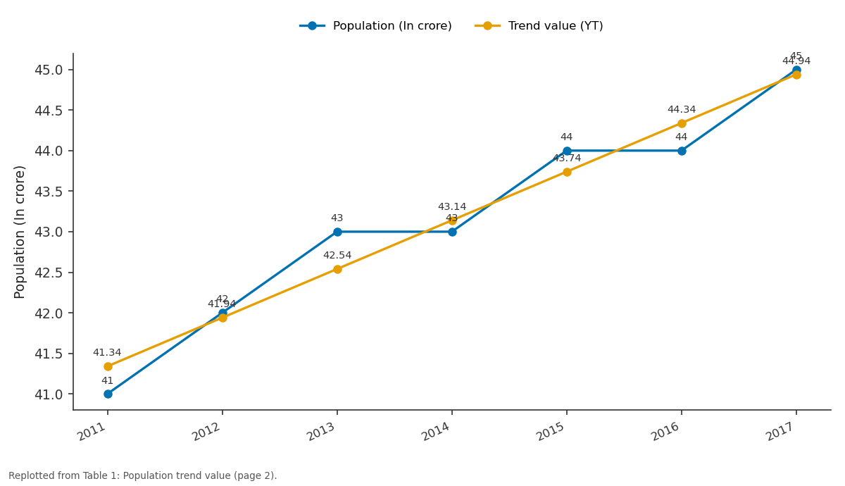
Population (In crore) and Trend value (YT): 2011 vs 2012 vs 2013 vs 2014 vs 2015
Replotted from Table 1 (page 2) of the original paper. Every bar is the paper's own table value.
View source evidence ↗Figures & tables
From the original paper Table 1
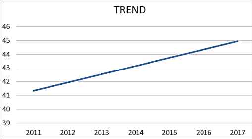 Figure 1
Introduction
The least square method is the process of estimating the best-fitting curve or line of best fit for a set of data by minimising the sum of the squares. During the process of finding the relation between two variables, the trend of outcomes are estimated quantitatively. This process is termed as regression analysis. The method of curve fitting is an approach to regression analysis. This method of fitting equations which approximates the curves to given raw data is the method of least square. It is quite obvious that the fitting of curves for a particular data set are not always unique. Thus, it is required to find a curve having a minimal deviation from all the measured data points. This is known as the best-fitting curve and is found by using the least-squares method. The least-squares method is a crucial statistical method to find a regression line or a best-fit line for the given set of data. This method is described by an equation with specific parameters. The method of least squares is generously used in evaluation and regression. In regression analysis, this method is said to be a standard approach for the approximation of sets of equations having more equations than the number of unknowns. The method of least squares actually defines the solution for the minimization of the sum of squares of deviations or the errors in the result of each equation. The least-squares method is often applied in data fitting. The best fit result is assumed to reduce the sum of squared errors or residuals which are stated to be the differences between the observed or experimental value and corresponding fitted value given in the model. ▪ The least squares method is a form of mathematical regression analysis that find the line of best fit for a database, providing a visual demonstration of the relationships between the data point. ▪ Each point of data is representative of the relationship between a known independent variable and unknown dependent variable ▪ The method yield very correct results if sufficiently good appraisal of the form of the function to the fitted data is obtained either by a security of the graphical plot of the values over time or by a theoretical understanding of the mechanism of the variable change.
Objective of the study
The objective of this research work is to estimate population trend by using last square method taking 7 years growth of population in Odisha that is from 2011 to 2017 using census data where population given in crores. The least square method enable us to estimate the trend values for all the given time periods in series. The fund equation can be used to estimate or predict the values of the variable for any period in future.
Significance of the study ▪ This method is completely free from personal bias of the analyst as it is very objective in nature. Anybody using this method is bound to fit the same type of straight line and find the same trend values fir the series. ▪ The least square method enables us to compare the trend values for all the given time period in the series. ▪ The trend equation can be used to estimate or predict the values of the variable for any period 't' in future. ▪ This method is the most popular and widely used for fitting mathematical function to a given set of observations.
Methodology
▪ The formula used for calculating method of least square.
▪ Statistical tabulation used for data.
Sources of data
▪ The secondary data obtained from census 2011 to 2017 (growth of population in Odisha) sources with internet.
Overview of the study Data
Overview of the study Data
Formula
The straight line trend is represented by the equation Y t = a + bt, where Yt are the trend values, a is the Y intercept on the value of Y when x = a, b represents the slope of line or the amount by which Y variable will change if x is increased or decreased by one unit, and x variable is the time period. In order to determine the value of the constant 'a' and 'b' following two equations called normal equations are to be solved.
Where 'n' is the number of time periods. For calculation, generally the mid-point of the given time series is taken as origin so that negative values of the first half of the series balance out the positive values of the second half and we get ∑x=0. When ∑x=0 the two normal equations will be reduced to a = .
Concluding remarks
Here, after that the estimated and mathematical calculation we conclude that from the above table estimation of population
Figures and tables from the paper
| Years | Population (In crore) | X | — | XY | Trend value (YT) |
|---|---|---|---|---|---|
| 2011 | 41 | -3 | 9 | -123 | 41.34 |
| 2012 | 42 | -2 | 4 | -84 | 41.94 |
| 2013 | 43 | -1 | 1 | -43 | 42.54 |
| 2014 | 43 | 0 | 0 | 0 | 43.14 |
| 2015 | 44 | 1 | 1 | 44 | 43.74 |
| 2016 | 44 | 2 | 4 | 88 | 44.34 |
| 2017 | 45 | 3 | 9 | 135 | 44.94 |
Table text extracted from the original PDF; superscript letters are shown inline. The original table image is below.
View original table image
References
0 in the original paperCited by 2
From OpenAlex, OpenCitations and reference lists read by Scinovex
- Estimation of Urban Water Needs with A Holistic Approach: The Case of Eskişehir, Türkiye ↗
Yıldırım Bayazıt · Water Conservation Science and Engineering · 2025
❝ 1 - Comparative study of methane emission quantification in Indonesian landfills ↗
Nita Citrasari, Ngurah Adi Mahendra Gautama, Diptya Adinda Larasati, Kholifatul Istiqomah, Dwi Ratri Mitha Isnadina, Sucipto Hariyanto et al. · Journal of Material Cycles and Waste Management · 2025
❝ 1