
Research article · 2021 · Full text
International Journal of Statistics and Applied MathematicsDerivation of confidence intervals for the difference, sum and ratio of coefficients of variation of normal distribution with a known ratio of variances
Volume 6(3) · Pages 24–29
Research areasSimulation Techniques and ApplicationsBayesian Methods and Mixture ModelsStatistical Distribution Estimation and Applications
Abstract
Author-writtenThis research paper proposes the confidence interval for the difference, sum and ratio of coefficients of variation of normal distribution with a known ratio of variance. The modified confidence intervals perform well for both the coverage probability and the expected length. These results are shown via Monte-Carlo simulation.
Summary
Source-checkedPlain-language reading of the full paper, prepared with AI and checked against the text. Each point links to the authors' own words.
Why it matters
- The coefficient of variation (CV) is a dimensionless statistical measure used to compare the dispersion of different variables by quantifying variability relative to the mean. View evidence ↗
- CV is applied across various fields, including economics, engineering, medicine, and science. View evidence ↗
- A known ratio of variances can occur in practice when two different instruments report the averaged response of the same object using different numbers of replicates. View evidence ↗
The question
- The study aims to propose confidence intervals for the sum, difference, and ratio of coefficients of variation for normal distributions when the ratio of variances is known. View evidence ↗
What they did
- The performance of several confidence intervals (CIGCI1, CIGCI2, CIROV1, CIROV2, and CIF) was evaluated using Monte-Carlo simulations. View evidence ↗
- The simulations consisted of 10,000 runs with a nominal confidence level set at 0.95. View evidence ↗
- The primary metrics used to evaluate the confidence intervals were their expected lengths and coverage probabilities. View evidence ↗
What they found
- The CIGCI1 confidence interval maintained coverage probabilities close to the nominal 0.95 level across all tested cases. View evidence ↗
- The coverage probabilities for the CIROV1 interval were unstable, decreasing as the variance ratio (c) increased. View evidence ↗
- The CIF interval based on Fieller's method produced wider intervals with coverage probabilities exceeding the nominal 0.95 level. View evidence ↗
- CIGCI2 demonstrated superior coverage probabilities compared to the MOVER method (CIROV2) across all sample sizes and variance ratios. View evidence ↗
What it means
- The authors recommend the Generalized Confidence Interval (GCI) method for constructing intervals for the sum, difference, and ratio of CVs because it consistently produces coverage probabilities near the nominal 0.95 level. View evidence ↗
Visual summary
3 visualsIllustrations explain the paper; charts are replotted from the paper's own table values.
Comparison of Confidence Interval Methods
AI-generated conceptual illustration (Normal distribution curves). It explains the idea and does not show study data.
View source evidence ↗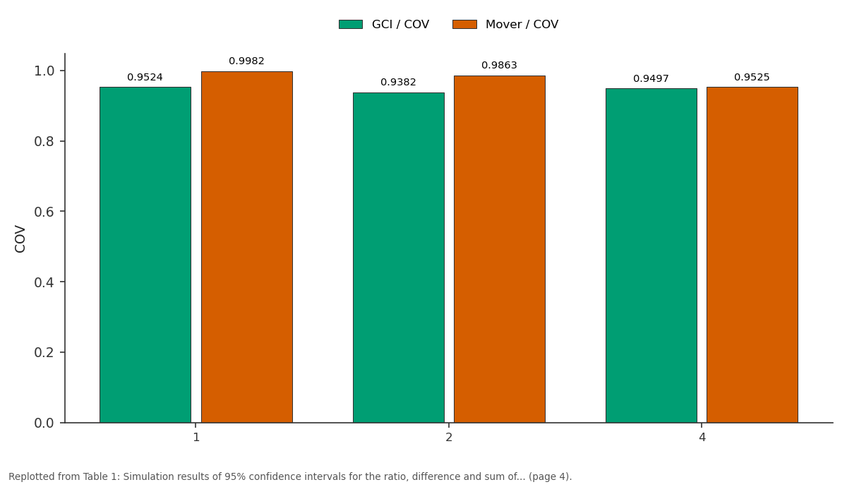
GCI / COV and Mover / COV: 1 vs 2 vs 4
Replotted from Table 1 (page 4) of the original paper. Every bar is the paper's own table value.
View source evidence ↗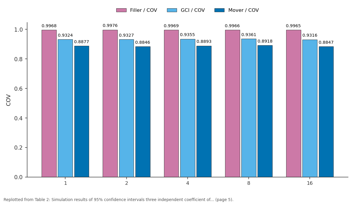
Filler / COV and GCI / COV and more: 1 vs 2 vs 4 vs 8 vs 16
Replotted from Table 2 (page 5) of the original paper. Every bar is the paper's own table value.
View source evidence ↗Figures & tables
From the original paper Table 1
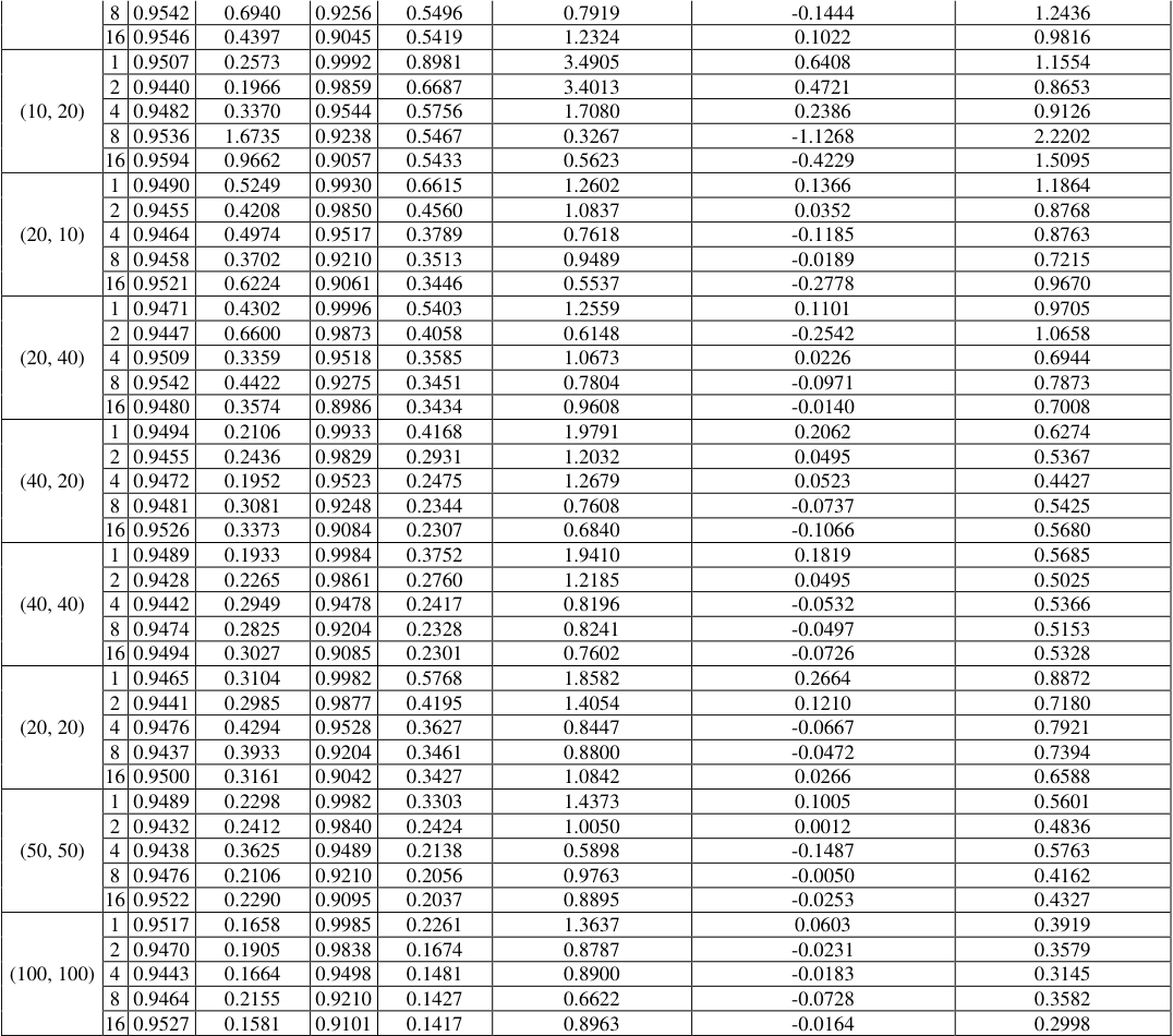 Table 2
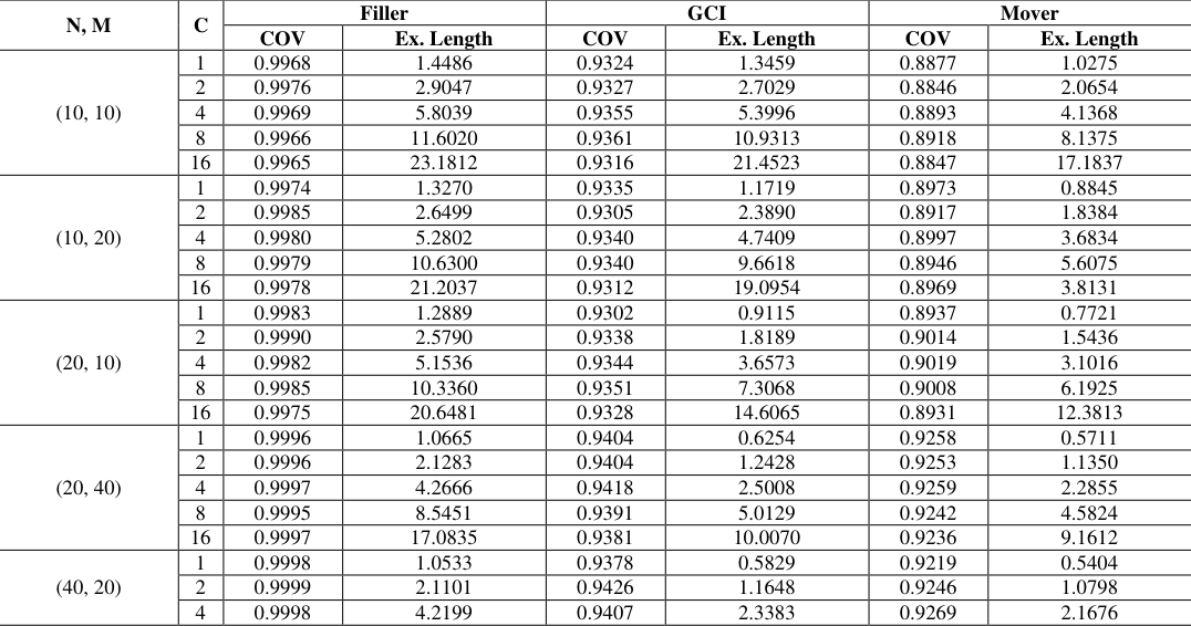 Table 2
Introduction
The coefficient of variation (CV) of a distribution is a dimensionless number that quantifies the degree of variability relative to the mean. It is a statistical measure for comparing the dispersion of several variables obtained by different units. The population coefficient of variation is defined as a ratio of the population standard deviation (𝜎) to the population mean (𝜇) given by 𝑘 = 𝜎/𝜇. The typical sample estimate of 𝑘 is given as 𝑘 ̂= 𝑆/𝑋 ̅ , where 𝑆 is the sample standard deviation, the square root of the unbiased estimator of population variance, and 𝑋 ̅ is the sample mean. The coefficient of variation has been widely used in many areas such as science, medicine, engineering, economics, and others. For example, the coefficient of variation was employed by Ahn (1995) [1] to analyze the uncertainty of fault trees. Gong and Li (1999) [6] assessed the strength of ceramics by using the coefficient of variation. Faber and Korn (1991) [4] applied the coefficient of variation as a way of including a measure of variation in the mean synaptic response of the central nervous system. The coefficient of variation has also been used to assess the homogeneity of bone test samples to help determine the effect of external treatments on the properties of bones as researched by Hammer et al (1995). Billings et al. (1993) [7,2] used the coefficient of variation to study the impact of socioeconomic status on hospital use in New York City. In finance and actuarial science, the coefficient of variation can be used as a measure of relative risk and a test of the equality of the coefficients of variation for two stocks as studied by Millerand and Karson (1977) [9] . Furthermore, Pyne et al. (2004) [10] studied the variability of the competitive performance of Olympic swimmers by using the coefficient of variation. The ratio of two independent coefficients of variation (CVs) is a particular problem in the estimation of two independent normally distributed random variables. This problem has previously appeared in the literature of Verrill and Johnson (2007) [15] . Their simulation results indicated that the performance of Verrill and Johnson confidence interval for the ratio of coefficients of variation by using the normal approximation worked quite well for small samples and the coverage probability of Verrill and Johnson confidence interval is not at least the nominal confidence levels. Recently, Wongkho et al. (2015) [17] have shown that the new confidence intervals based on the generalized confidence interval (GCI) of Weerahandi (1993) [16] and the new confidence interval based on the method of variance estimates recovered from the confidence limits (Mover) described by Donner and Zou (2010) [3] are better than Verrill and Johnson's confidence interval. As a result, they recommended both methods for constructing the confidence interval for the ratio of coefficients of variation. In this paper, this research study considers not only the ratio of the CVs of normal distribution but also the difference and sum between CVs when we know a ratio of variances. Schechtman and Sherman (2007) [12] described a situation of a known ratio of variances arises in practice when two instruments report (averaged) response of the same object based on a difference number of replicates. If the two instruments have the same precision for a single measurement, then the ratio of the variance of the responses is known, and it is simply the ratio of the number of replicates going into each response. They finally proposed a t-test statistic, which has an exact t-distribution with n+m-2 degrees of freedom, compared to the Satterthwaite's t-test statistic. They found that their proposed test has more power than an existing Satterthwaite's test. However, they did not investigate the coverage probability and the expected length of the confidence intervals for the difference and the ratio of CVs when the ratio of variances is known.
Confidence intervals for the difference, sum and ratio of coefficients of variation of normal distribution with a known ratio of variance
be estimators of the population means and population variances of 𝑋 𝑎𝑛𝑑 𝑌 respectively. Then the construction of the confidence interval for the difference, sum and ratio of coefficients of variation are supposed to be 𝜂
In some cases, when the ratio of variances are known as explained by Shechman and Sherman (2007) [12] and further expanded by the author, the parameter of interest, 𝜂 = 𝜃 1 𝜃 2 ⁄
. Also, the parameter of 𝛿 = 𝜃 1 -𝜃 2 reduces to 𝛿 = 𝜎 1 𝜇 1 ⁄ -
The generalized confidence interval (GCI)
The Generalized Confidence Interval (GCI) for the difference, sum and ratio between the coefficients of variation of normal distributions is being presented in this subsection based on the works of Weerahandi (1993) [16] . Weerahandi (1993) [16] defined a generalized pivot (GP) as a statistic that has a distribution free of unknown parameters and an observed value of a generalized pivotal quantity does not depend on nuisance parameters. In a general setting, a generalized pivot can be defined as follows: Let X be a random quantity having a density function 𝑓(𝑋, 𝜉) 𝑤ℎ𝑒𝑟𝑒 𝜉 = {𝜃, 𝜏} are unknown parameters; 𝜃 is the parameter of interest and 𝜏 is a nuisance parameter. Let 𝑥 be the observed value of 𝑋. In the procedure to construct the confidence interval for 𝜃, we start with a generalized pivotal quantity 𝑅(𝑋, 𝑥, 𝜉) which is a function of random variable 𝑋, its observed value 𝑥 and the parameter 𝜉. Also, 𝑅(𝑋, 𝑥, 𝜉) is required to satisfy the following conditions: Condition 1: For fix 𝑥, a probability distribution of 𝑅(𝑋, 𝑥, 𝜉) is free of unknown parameters.
Condition 2:
The observed pivot, which is defined as 𝑅(𝑥, 𝑥, 𝜉),, does not depend on nuisance parameter. Now, we construct confidence interval for 𝜂 = 𝜃 1 𝜃 2 ⁄ where 𝜃 1 = 𝜎 1 𝜇 1 ⁄ 𝑎𝑛𝑑 𝜃 2 = 𝜎 2 𝜇 2 ⁄ , and the ratio of variances
is straightforward to see that:
Using equation (1), we can define generalized pivotal quantity as:
where 𝑠 1 , 𝑠 2 , 𝑥̅ 𝑎𝑛𝑑 𝑦 ̅ are the observed values of 𝑆 1 , 𝑆 2 , 𝑋 ̅ 𝑎𝑛𝑑 𝑌 ̅ respectively.
It is easy to see that 𝑄(𝑋, 𝑌, 𝑥, 𝑦, 𝜉), 𝑃(𝑋, 𝑌, 𝑥, 𝑦, 𝜉) 𝑎𝑛𝑑 𝑅(𝑋, 𝑌, 𝑥, 𝑦, 𝜉) satisfy Conditions 1 and 2 above. Therefore, the 100(1 -𝛼)% generalized confidence interval for 𝜂, Ω 𝑎𝑛𝑑 𝛿 are respectively:
are the (1 -𝛼 2 ⁄ )th percentile for 𝑄(𝑋, 𝑌, 𝑥, 𝑦, 𝜉), 𝑃(𝑋, 𝑌, 𝑥, 𝑦, 𝜉) and 𝑅(𝑋, 𝑌, 𝑥, 𝑦, 𝜉) respectively.
The method of variance estimates recovery (Mover)
Zou, Huo and Taleban (2009), and Donner and Zhou (2010) [18,3] as researchers proposed a simple confidence interval for the sum of the parameters 𝜃 1 𝑎𝑛𝑑 𝜃 2 (𝑡ℎ𝑎𝑡 𝑖𝑠, 𝜃 1 + 𝜃 2 ) is in the form of:
where 𝜃 1 ̂ 𝑎𝑛𝑑 𝜃 2 ̂ are the estimates of the parameters 𝜃 1 𝑎𝑛𝑑 𝜃 2 respectively. Suppose 𝐶𝐼 0 = [𝐿, 𝑈] is the confidence interval for 𝜃 1 + 𝜃 2 . Furthermore, Zou, Huo and Taleban (2009), and Donner and Zhou (2010) [18,3] also found that:
where 𝜃 1 𝜖(𝑙 1 , 𝑢 1 ) 𝑎𝑛𝑑 𝜃 2 𝜖(𝑙 2 , 𝑢 2 ), and the confidence interval for 𝜃 1 -𝜃 2 is 𝜃 1 + (-𝜃 2 ). It is noted that the confidence interval for -𝜃 2 is (-𝑢 2 , 𝑙 2 ) and it replaced 𝜃 2 𝜖(-𝑢 2 , 𝑙 2 ) in equation ( 4). Therefore the confidence interval for 𝜃 1 -𝜃 2 is:
Now, we set 𝜃 1 = 𝐾 1 = 𝜎 1 𝜇 1 , ⁄ 𝜃 2 = 𝐾 2 = 𝜎 2 𝜇 2 , ⁄ 𝜃 ̂1 = 𝐾 ̂1 = 𝑆 1 𝑋, ⁄ 𝜃 ̂2 = 𝐾 ̂2 = 𝑆 2 𝑌, ⁄ and putting these in equation ( 5), the confidence interval for 𝜃 1 -𝜃 2 is as follows:
Donner and Zhou (2010) [3] again proposed the confidence interval for the ratio of parameters, 𝜃 1 /𝜃 2 , by using the method of variance estimates recovery in 2010. They constructed the confidence interval for 𝜃 3 /𝜃 4 by using the confidence limits 𝑙 𝑖 , 𝑢 𝑖 , 𝑖 = 3,4 where 𝑙 𝑖 , 𝑢 𝑖 are the 100 (1 -𝛼 2)% ⁄ two-sided confidence intervals for 𝜃 𝑖 . Then, the confidence interval for 𝜃 3 /𝜃 4 is given by 𝜂 𝐿 , 𝜂 𝑈 , where:
Following the research of Donner and Zhou (2010) [3] , the confidence interval for 𝛿 = 𝜎 1 𝜇 1 ⁄ -𝑐 -1 𝜎 1 𝜇 2 ⁄ is starting from the following: A confidence interval for 𝜃 1 = 𝜎 1 𝜇 1 ⁄ which as Mahmoudvand and Hassani (2009) [8] is:
and 𝜃 ̂1 = 𝑘 ̂1, 𝐾 ̂1 = 𝑆 1 /𝑋 ̅ Following with a confidence interval for 𝑐 -1 𝜎 1 𝜇 2 ⁄ which is: ) and 𝑙 4 . 𝑢 4 = 𝑌 ̅ -𝑧 1-𝛼 2 ⁄ 𝑆 2 /√𝑚 ≤ 𝜇 2 ≤ 𝑌 ̅ + 𝑧 1-𝛼 2 ⁄ 𝑆 2 /√𝑚, 𝜃 ̂2 = 𝑐 -1 𝑆 1 /𝑌 ̅ , 𝜃 ̂3 = 𝑐 -1 𝑆 1 , 𝜃 ̂4 = 𝑌 ̅ , putting these 𝑙 3 . 𝑢 3 and 𝑙 4 . 𝑢 4 in equations ( 6) and ( 7), we then have 𝑙 2 . 𝑢 2 = 𝜂 𝐿 , 𝜂 𝑈 , and finally putting 𝑙 1 . 𝑢 1 and 𝑙 2 . 𝑢 2 in equation ( 5), we then have a confidence interval for 𝛿 = 𝜎 1 𝜇 1 ⁄ -𝑐 -1 𝜎 1 𝜇 2 ⁄ . This confidence interval is called 𝐶𝐼 𝑟𝑜𝑣1 .
The confidence interval for 𝜂 =
is therefore constructed from equations ( 6) and ( 7) by replacing:
The confidence interval for 𝜽 based on fieller's method
In the construction of the confidence interval for 𝜂 = 𝑐 𝜇 2 𝜇 1 ⁄ by the application of Fieller's method (1954) [5] :
a statistics √(𝑛 + 𝑚 -2) (𝑛 + 𝑚) ⁄ 𝑇 follows t-distribution with (n+m-2) degrees of freedom. A 100(1-α)% confidence interval for θ, by solving equation ( 8), which is:
where 𝑡 1-𝛼 2 ⁄ is the (1 -𝛼 2 ⁄ )th percentile of t-distribution with 𝑛 + 𝑚 -2 degrees of freedom. Note that T has an exact tdistribution with 𝑛 + 𝑚 -2 degrees of freedom. The confidence interval 𝐶𝐼 𝐹 * * can be transformed into:
Results of simulation studies
Extensive studies and evaluations were done on the performance of all confidence intervals: 𝐶𝐼 𝑔𝑐𝑖1 , 𝐶𝐼 𝑔𝑐𝑖2 , 𝐶𝐼 𝑟𝑜𝑣1 , 𝐶𝐼 𝑟𝑜𝑣2 , 𝐶𝐼 𝐹 via Monte-Carlo simulation. The simulation studies are carried out to evaluate the coverage probabilities and expected lengths of each confidence interval. The number of simulation runs is equal to 10,000 and the design value of the nominal confidence level is 0.95. For the generalized pivotal approach, in each of 10,000 simulations, 500 pivotal quantities are used. All data are generated from normal distribution with means 𝜇 1 = 𝜇 2 = 1 and standard deviations 𝜎 1 = 𝜎 2 = 1, 𝑐 = [1,2,4,8,16] and sample sizes (𝑛, 𝑚) = (10,20,40,100). The results were performed using a program written in the R statistic software. The simulation results are shown in Tables 1 and2. As seen in Table 1, the confidence interval 𝐶𝐼 𝑔𝑐𝑖1 has coverage probabilities approximately nominal confidence level of 0.95 in all cases, but the coverage probabilities of the confidence interval 𝐶𝐼 𝑟𝑜𝑣1 are slightly decreasing from the nominal value as 𝑐 is increasing. This means the coverage probabilities of the confidence interval 𝐶𝐼 𝑟𝑜𝑣1 is not stable, that is, it is depending on the values of 𝑐. Therefore, the confidence interval 𝐶𝐼 𝑔𝑐𝑖1 is chosen for the ratio of coefficient of variations (CVs) with a known ratio of variances 𝜂 = 𝜃 1 𝜃 2 ⁄ . From Table 2, the confidence interval 𝐶𝐼 𝐹 using the Fieller's method has produced a wider confidence interval as usual since coverage probabilities of this confidence interval are over the nominal level at 0.95. Therefore, the confidence interval 𝐶𝐼 𝐹 is not considered. The confidence interval 𝐶𝐼 𝑔𝑐𝑖2 have much coverage probabilities than the confidence interval for MOVER method, 𝐶𝐼 𝑟𝑜𝑣2 for all sample sizes and values of c. Therefore, the confidence interval 𝐶𝐼 𝑔𝑐𝑖2 is chosen for the difference between CVs when we know a ratio of variances. The simulation studies was as well extended to the difference and sum of variances.
| N, M | C | Filler | — | GCI | — | Mover | — |
|---|---|---|---|---|---|---|---|
| COV | Ex. Length | COV | Ex. Length | COV | Ex. Length | ||
| (10, 10) | 1 | 0.9968 | 1.4486 | 0.9324 | 1.3459 | 0.8877 | 1.0275 |
| 2 | 0.9976 | 2.9047 | 0.9327 | 2.7029 | 0.8846 | 2.0654 | |
| 4 | 0.9969 | 5.8039 | 0.9355 | 5.3996 | 0.8893 | 4.1368 | |
| 8 | 0.9966 | 11.6020 | 0.9361 | 10.9313 | 0.8918 | 8.1375 | |
| 16 | 0.9965 | 23.1812 | 0.9316 | 21.4523 | 0.8847 | 17.1837 | |
| (10, 20) | 1 | 0.9974 | 1.3270 | 0.9335 | 1.1719 | 0.8973 | 0.8845 |
| 2 | 0.9985 | 2.6499 | 0.9305 | 2.3890 | 0.8917 | 1.8384 | |
| 4 | 0.9980 | 5.2802 | 0.9340 | 4.7409 | 0.8997 | 3.6834 | |
| 8 | 0.9979 | 10.6300 | 0.9340 | 9.6618 | 0.8946 | 5.6075 | |
| 16 | 0.9978 | 21.2037 | 0.9312 | 19.0954 | 0.8969 | 3.8131 | |
| (20, 10) | 1 | 0.9983 | 1.2889 | 0.9302 | 0.9115 | 0.8937 | 0.7721 |
| 2 | 0.9990 | 2.5790 | 0.9338 | 1.8189 | 0.9014 | 1.5436 | |
| 4 | 0.9982 | 5.1536 | 0.9344 | 3.6573 | 0.9019 | 3.1016 | |
| 8 | 0.9985 | 10.3360 | 0.9351 | 7.3068 | 0.9008 | 6.1925 | |
| 16 | 0.9975 | 20.6481 | 0.9328 | 14.6065 | 0.8931 | 12.3813 | |
| (20, 40) | 1 | 0.9996 | 1.0665 | 0.9404 | 0.6254 | 0.9258 | 0.5711 |
| 2 | 0.9996 | 2.1283 | 0.9404 | 1.2428 | 0.9253 | 1.1350 | |
| 4 | 0.9997 | 4.2666 | 0.9418 | 2.5008 | 0.9259 | 2.2855 | |
| 8 | 0.9995 | 8.5451 | 0.9391 | 5.0129 | 0.9242 | 4.5824 | |
| 16 | 0.9997 | 17.0835 | 0.9381 | 10.0070 | 0.9236 | 9.1612 | |
| (40, 20) | 1 | 0.9998 | 1.0533 | 0.9378 | 0.5829 | 0.9219 | 0.5404 |
| 2 | 0.9999 | 2.1101 | 0.9426 | 1.1648 | 0.9246 | 1.0798 | |
| 4 | 0.9998 | 4.2199 | 0.9407 | 2.3383 | 0.9269 | 2.1676 |
Table text extracted from the original PDF; superscript letters are shown inline. The original table image is below.
View original table image
| — | 8 | 0.9542 | 0.6940 | 0.9256 | 0.5496 | 0.7919 | -0.1444 | 1.2436 |
|---|---|---|---|---|---|---|---|---|
| 16 | 0.9546 | 0.4397 | 0.9045 | 0.5419 | 1.2324 | 0.1022 | 0.9816 | |
| (10, 20) | 1 | 0.9507 | 0.2573 | 0.9992 | 0.8981 | 3.4905 | 0.6408 | 1.1554 |
| 2 | 0.9440 | 0.1966 | 0.9859 | 0.6687 | 3.4013 | 0.4721 | 0.8653 | |
| 4 | 0.9482 | 0.3370 | 0.9544 | 0.5756 | 1.7080 | 0.2386 | 0.9126 | |
| 8 | 0.9536 | 1.6735 | 0.9238 | 0.5467 | 0.3267 | -1.1268 | 2.2202 | |
| 16 | 0.9594 | 0.9662 | 0.9057 | 0.5433 | 0.5623 | -0.4229 | 1.5095 | |
| (20, 10) | 1 | 0.9490 | 0.5249 | 0.9930 | 0.6615 | 1.2602 | 0.1366 | 1.1864 |
| 2 | 0.9455 | 0.4208 | 0.9850 | 0.4560 | 1.0837 | 0.0352 | 0.8768 | |
| 4 | 0.9464 | 0.4974 | 0.9517 | 0.3789 | 0.7618 | -0.1185 | 0.8763 | |
| 8 | 0.9458 | 0.3702 | 0.9210 | 0.3513 | 0.9489 | -0.0189 | 0.7215 | |
| 16 | 0.9521 | 0.6224 | 0.9061 | 0.3446 | 0.5537 | -0.2778 | 0.9670 | |
| (20, 40) | 1 | 0.9471 | 0.4302 | 0.9996 | 0.5403 | 1.2559 | 0.1101 | 0.9705 |
| 2 | 0.9447 | 0.6600 | 0.9873 | 0.4058 | 0.6148 | -0.2542 | 1.0658 | |
| 4 | 0.9509 | 0.3359 | 0.9518 | 0.3585 | 1.0673 | 0.0226 | 0.6944 | |
| 8 | 0.9542 | 0.4422 | 0.9275 | 0.3451 | 0.7804 | -0.0971 | 0.7873 | |
| 16 | 0.9480 | 0.3574 | 0.8986 | 0.3434 | 0.9608 | -0.0140 | 0.7008 | |
| (40, 20) | 1 | 0.9494 | 0.2106 | 0.9933 | 0.4168 | 1.9791 | 0.2062 | 0.6274 |
| 2 | 0.9455 | 0.2436 | 0.9829 | 0.2931 | 1.2032 | 0.0495 | 0.5367 | |
| 4 | 0.9472 | 0.1952 | 0.9523 | 0.2475 | 1.2679 | 0.0523 | 0.4427 | |
| 8 | 0.9481 | 0.3081 | 0.9248 | 0.2344 | 0.7608 | -0.0737 | 0.5425 | |
| 16 | 0.9526 | 0.3373 | 0.9084 | 0.2307 | 0.6840 | -0.1066 | 0.5680 | |
| (40, 40) | 1 | 0.9489 | 0.1933 | 0.9984 | 0.3752 | 1.9410 | 0.1819 | 0.5685 |
| 2 | 0.9428 | 0.2265 | 0.9861 | 0.2760 | 1.2185 | 0.0495 | 0.5025 | |
| 4 | 0.9442 | 0.2949 | 0.9478 | 0.2417 | 0.8196 | -0.0532 | 0.5366 | |
| 8 | 0.9474 | 0.2825 | 0.9204 | 0.2328 | 0.8241 | -0.0497 | 0.5153 | |
| 16 | 0.9494 | 0.3027 | 0.9085 | 0.2301 | 0.7602 | -0.0726 | 0.5328 | |
| (20, 20) | 1 | 0.9465 | 0.3104 | 0.9982 | 0.5768 | 1.8582 | 0.2664 | 0.8872 |
| 2 | 0.9441 | 0.2985 | 0.9877 | 0.4195 | 1.4054 | 0.1210 | 0.7180 | |
| 4 | 0.9476 | 0.4294 | 0.9528 | 0.3627 | 0.8447 | -0.0667 | 0.7921 | |
| 8 | 0.9437 | 0.3933 | 0.9204 | 0.3461 | 0.8800 | -0.0472 | 0.7394 | |
| 16 | 0.9500 | 0.3161 | 0.9042 | 0.3427 | 1.0842 | 0.0266 | 0.6588 | |
| (50, 50) | 1 | 0.9489 | 0.2298 | 0.9982 | 0.3303 | 1.4373 | 0.1005 | 0.5601 |
| 2 | 0.9432 | 0.2412 | 0.9840 | 0.2424 | 1.0050 | 0.0012 | 0.4836 | |
| 4 | 0.9438 | 0.3625 | 0.9489 | 0.2138 | 0.5898 | -0.1487 | 0.5763 | |
| 8 | 0.9476 | 0.2106 | 0.9210 | 0.2056 | 0.9763 | -0.0050 | 0.4162 | |
| 16 | 0.9522 | 0.2290 | 0.9095 | 0.2037 | 0.8895 | -0.0253 | 0.4327 | |
| (100, 100) | 1 | 0.9517 | 0.1658 | 0.9985 | 0.2261 | 1.3637 | 0.0603 | 0.3919 |
| 2 | 0.9470 | 0.1905 | 0.9838 | 0.1674 | 0.8787 | -0.0231 | 0.3579 | |
| 4 | 0.9443 | 0.1664 | 0.9498 | 0.1481 | 0.8900 | -0.0183 | 0.3145 | |
| 8 | 0.9464 | 0.2155 | 0.9210 | 0.1427 | 0.6622 | -0.0728 | 0.3582 | |
| 16 | 0.9527 | 0.1581 | 0.9101 | 0.1417 | 0.8963 | -0.0164 | 0.2998 |
Table text extracted from the original PDF; superscript letters are shown inline. The original table image is below.
View original table image
| N, M | C | GCI | — | Mover | — | Ratio (Mover/GCI) | Difference (Mover - GCI) | SUM (Mover + GCI) |
|---|---|---|---|---|---|---|---|---|
| COV | Ex. Length | COV | Ex. Length | |||||
| (10, 10) | 1 | 0.9524 | 1.9095 | 0.9982 | 0.9754 | 0.5108 | -0.9341 | 2.8849 |
| 2 | 0.9382 | 0.2344 | 0.9863 | 0.6992 | 2.9829 | 0.4648 | 0.9336 | |
| 4 | 0.9497 | 0.4532 | 0.9525 | 0.5897 | 1.3012 | 0.1365 | 1.0429 |
Table text extracted from the original PDF; superscript letters are shown inline. The original table image is below.
View original table image
Conclusion
The confidence intervals for the difference, sum and ratio of coefficients of variation of normal distribution with a known ratio have been studied. The performances of theses confidence intervals were assessed in terms of coverage probabilities and expected lengths through simulation studies. The simulation results indicated that the GCI method produce the coverage probability close to the nominal confidence level, 0.95 for all the sample sizes and values of c. Therefore, the recommendation for the difference, sum and ratio of CVs when the ratio of variances is used to construct the confidence intervals is suggested.
References
18 in the original paper- Ahn K. "On the use of coefficient of variation for uncertainty analysis in fault tree analysis" Reliability Engineering and System Safety 1995;47(3):229-230.
- Billings J, Zeitel L, Lukomnik J, Carey TS, Blank AE, Newman L. "Impact of socioeconomic status on hospital use in New York City" Health Affairs 1993;12(1):162-173.
- Donner A, Zou GY. Closed-form confidence intervals for functions of the normal and standard deviation. Statistical Methods in Medical Research 2010;21(4):347-359.
- Faber DS, Korn H. "Applicability of the coefficient of variation method for analyzing synaptic plasticity" Biophysical Journal 1991;60(5):1288-1294.
- Fieller EC. A fundamental formula in the statistics of biological essay and application. Q. J. Pharm. Pharmacol 1954;17:117223.
- Gong J, Li Y. "Relationship between the Estimated Weibull Modulus and the Coefficient of Variation of the Measured Strength for Ceramics" Journal of the American Ceramic Society 1999;82(2):449-452.
- Hammer AJ, Strachan JR, Black MM, Ibbotson C, Elson RA. "A new method of comparative bone strength measurement" Journal of Medical Engineering and Technology 1995;19(1):1-5.
- Mahmoudvand R, Hassani H. Two new confidence intervals for the coefficient of variation in a normal distribution. Journal of Applied Statistics 2009;36(4):429-442.
- Millerand EG, Karson MJ. "Testing the equality of two coefficients of variation" in American Statistical Association: Proceedings of the Business and Economics Section 1977;I:278-283.
- Pyne DB, Trewin CB, Hopkins WG. "Progression and variability of competitive performance of Olympic swimmers" Journal of Sports Sciences 2004;22(7):613-620.
- R Development Core Team, R: a language and environment for statistical computing, R Foundation for Statistical Computing 2005.
- Senechtman E, Sherman M. The two-sample t-test with a known ratio of variances. Statistical Methodology 2007;4:508-514.
- Smithson M. "Correct confidence intervals for various regression effect sizes and parameters: the importance of non-central distributions in computing intervals" Educational and Psychological Measurement 2001;61(4):605-632.
- Thompson B. "What future quantitative social science research could look like: confidence intervals for effect sizes" Educational Researcher 2002;31(3):25-32.
- Verrill S, Johnson RA. Confidence bounds and hypothesis tests for normal distribution coefficients of variation. Communication in Statistics-Theory and Method 2007;36:2187-2206.
- Weeahandi S. Generalized Confidence Interval. Journal of the American Statistical Association 1993;88(423):899-905.
- Wongkhao A, Niwitpong S, Niwitpong SA. Confidence interval for the ratio of two independent coefficients of variation of normal distribution. Far East Journal of Mathematical Sciences 2015;98:741-757.
- Zou GY, Huo CY, Taleban J. Simple confidence intervals for lognormal means and their differences with exponential applications. Environmetrics 2009;20:172-180.