
Research article · 2020 · Full text
International Journal of Veterinary Sciences and Animal HusbandryApplication of artificial neural network (ann) to evaluate extend of non-linearity among explanatory variables within and between genotypes and phenotypes
Volume 5(3) · Pages 21–26
Research areasGenetic and phenotypic traits in livestockEffects of Environmental Stressors on LivestockGenetic Mapping and Diversity in Plants and Animals
Abstract
Author-writtenArtificial neural networks (ANN) have been described as an additional model for marker-based genomic predictions of complex traits in the field of animal breeding. This is because of their ability to accommodate noisy, nonlinearity in data set and they make decisions based on prior knowledge. The focus of this study was, therefore, to evaluate the extent of non-linearity among explanatory variables within and between genotypes and phenotypes using ANN. A feedforward ANN was adopted with different number of neurons where Levenberg-Marquardt back-propagation algorithm was used to train the network. The construction and training of the network were done with matrix laboratory (MATLAB). Mean absolute error (MAE) and Pearson’s correlation coefficients (R) were used to measure the ANN predictive performance as a measure of extent of non-linearity among explanatory variables within and between genotypes and phenotypes. The results showed that the ANN models differed in predictive performance depending on the number of neurons in the hidden layer, for instance the neural network with one hidden layer containing 10 neurons in the hidden layer yielded high R-value of 0.86 and MAE of 2.98E-3. When the network dimension was increased to 16 neurons the performance decreased to 0.67 for R and MAE increased to 7.73E-2. After a further increase of neurons to 32 the model yielded R value of 0.27 and MAE of 7.60E-2. The benchmark model for this study had an R of 0.77 and MAE of 5.72. These results imply that a model with 10 neurons is enough to handle nonlinearity in data set thus chosen as the best nonlinear model. This is because dimension reduction of neurons in the hidden layer led to higher, more accurate and more consistent predictions for growth rate. In comparison to linear model, the best nonlinear model performed better though the more complex non-linear architectures with 16 and 32 neurons could not outperform the linear ANN. Thus, linear models can as well produce reliable results for making genomic predictions.
Summary
Source-checkedPlain-language reading of the full paper, prepared with AI and checked against the text. Each point links to the authors' own words.
Why it matters
- Artificial neural networks (ANN) are useful for genomic predictions of complex traits in animal breeding because they can handle noisy data and non-linear relationships. View evidence ↗
- Predicting animal performance early is critical for increasing genetic progress by reducing generation intervals and improving selection intensity. View evidence ↗
- Standard linear algebraic methods cannot account for all the linear and non-linear interactions between environment, management, and seasons that affect production traits. View evidence ↗
The question
- The study aimed to use ANNs to evaluate the extent of non-linearity between genotypes and phenotypes. View evidence ↗
What they did
- The research used 394 birds from four Chinese indigenous chicken breeds, including low-body-weight (Chahua and Silkie) and intermediate/high-body-weight (Beard and Langshan) breeds. View evidence ↗
- After quality control, 46,211 SNPs were initially retained, which was further reduced to 26,698 markers for analysis after removing those with 50% missing genotypes. View evidence ↗
- The dataset was split into training and test sets, with the training portion further divided into 70% for training and 30% for validation. View evidence ↗
- The networks were trained using the Levenberg-Marquardt back-propagation algorithm with a maximum of 2,000 epochs. View evidence ↗
- Predictive performance was measured using Mean Absolute Error (MAE) and Pearson’s correlation coefficients (R). View evidence ↗
What they found
- The ANN model with 10 neurons in one hidden layer performed best, achieving an R-value of 0.86 and an MAE of 2.98E-3. View evidence ↗
- Increasing the network to 16 neurons decreased performance, with R dropping to 0.67 and MAE increasing to 7.73E-2. View evidence ↗
- Further increasing the network to 32 neurons led to a significant performance drop, with an R-value of 0.27 and an MAE of 7.60E-2. View evidence ↗
- The linear benchmark model (one neuron in the hidden layer) achieved an R of 0.77 and an MAE of 5.72E-3. View evidence ↗
What it means
- The authors recommend using a single hidden layer with 10 neurons for efficient handling of non-linearity in growth rate predictions. View evidence ↗
- The authors conclude that linear models can also provide reliable results for genomic predictions. View evidence ↗
- Increasing network dimensionality can lead to overfitting or underfitting as the model may learn irrelevant details of the dataset. View evidence ↗
Figures & tables
From the original paper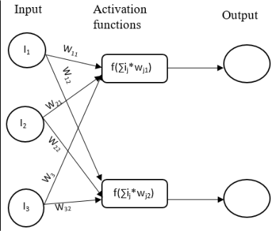 Figure 1
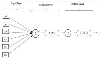 Figure 3
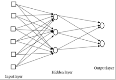 Figure 2
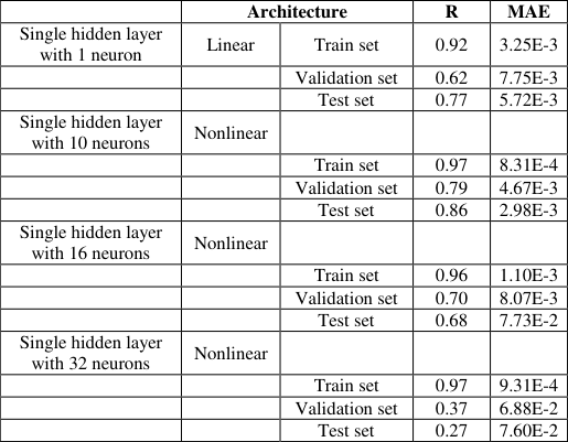 Table 1
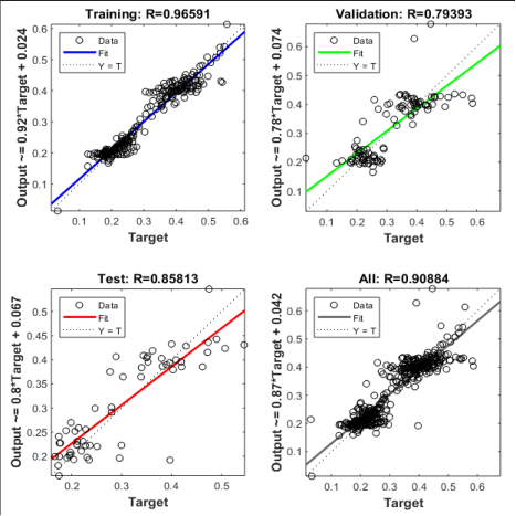 Figure 1
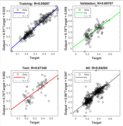 Figure 2
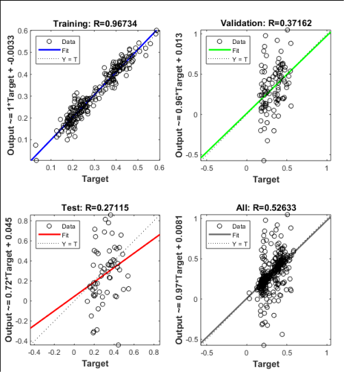 Figure 3
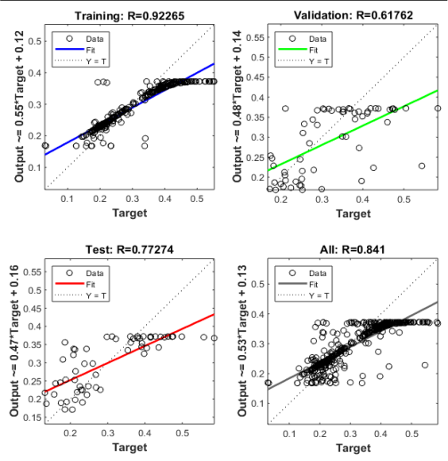 Figure 4
Introduction
Artificial neural networks (ANN) is a mathematical model which mimic the way the biological neural network of human brain works. It has the ability to learn from experience to improve its performance and to adapt themselves to changes in the environment (Njubi et al., 2010) [14] . The ANN architecture comprises of the input, hidden and output layers. These layers are connected by synapses denoted as weights, the weights are then multiplied by input to give the desired output. For many decades ANNs have been successfully applied in fields of engineering, medical diagnosis, economic predictions and image recognition (Gorgulu, 2012) [7] . Consequently, ANN has proven to be a powerful modelling tool in comparison with other conventional models because it has an ability to predict outcome of nonlinear and noisy data (Ehret et al., 2015) [3] . Even though ANN model has shown a lot of inspiring success in prediction of outcome, its application in animal breeding is still scarce (Gorgulu, 2012) [7] , considering huge dataset available to be analyzed in this field. The first application of ANNs in the field of animal breeding was by Macrossam et al. (1999) [12] , where they used ANN as a method for optimizing mating allocation to maximize production traits in Australian dairy industry. Since then the development and applications of ANNs in animal breeding are increasing steadily, owing their flexibility in classification, pattern recognition, prediction and Forecasting, process control, optimization and decision support (Hanrahan, 2011) [9] . Artificial neural networks have been described as an additional model in performance prediction in the field of animal breeding (Gianola et al., 2011) [5] . It has been pointed out to be a promising tool for molecular marker-based genomic predictions of complex traits in animals (Ehret, et al., 2015) [5] . Early prediction of performance is important in reducing generation intervals, making management decisions and increasing intensity of selection thus greater genetic progress (Gorgulu, 2012) [7] . Therefore, phenotypic prediction from genotypes plays an important role in identifying and selecting superior candidates to be used in a breeding program, this facilitates early utilization of best genotypes for economic gain. Genomic prediction is always applied early in a breeding program as a way to increase the overall selection pressure thus increasing the rate of genetic gain (Mcdowell, 2016) [13] . Selection and mating strategies are important in designing a breeding program and have been adopted successfully in developed countries unlike in developing countries where application of these practices is still inadequate (Njubi et al., 2010) [14] . Breeding programs in the tropics are based primarily on performance based on production traits, because they are readily available and often used to measure of economic profitability of an enterprise (Njubi et al., 2010) [14] . Production traits such as milk production are affected by linear and nonlinear interactions between environmental conditions, management, and seasons. The commonly used linear algebraic methods (Mrode, 2014) possess inherent restrictions which makes them not able to consider all these interactions. Artificial neural networks have been reported to possess an ability to accommodate noisy data, linear and nonlinear relationships between variables and interactions between explanatory variables and finally ambiguity of data from environmental influence (Ehret et al., 2015; Gonzalez-Camacho et al., 2012) [3,6] . They are also known for making accurate selection decisions based on prior knowledge of the outcome (Hosseinia et al., 2007) [10] . The focus of this study was, therefore, to evaluate the extent of non-linearity among explanatory variables within and between genotypes and phenotypes using ANN.
Materials and methods
Materials and methods
Data source
The data used for this study were obtained from a widegenome study in four Chinese indigenous chicken breeds (Yuan et al., 2018) [18] . The study used 394 birds from four indigenous breeds consisting of two typical low-body-weight breeds (Chahua chicken and Silkie chicken) and two intermediate and high body-weight breeds (Beard chicken and Langshan chicken). The birds were randomly selected from the original conserved population and bred by performing artificial insemination of hens with sperm pools. The obtained fertilized eggs were incubated and the chicks were of an approximately equal number of cocks and hens. The hens and cocks of the different breeds were phenotyped for body weight. Live body weight (BW) was measured at hatch and every week until 15 weeks of age.
Sample collection, DNA extraction and genotyping
Blood samples were collected from 394 birds at 15 weeks of age. The DNA extraction was done using the phenolchloroform method and diluted to 50 ng/ml. Genotyping was performed using Illumina 60K Chicken SNP BeadChip (Groenen et al., 2011) [8] . Quality control was conducted on all birds (after quality control of their phenotypic records) across four breeds by customized scripts in R software version 3.3.0 (R Core Team, 2013). Single-nucleotide polymorphisms (SNPs) filtering were done using the following criteria: individual samples were excluded with call rates < 0.9 and minor allele frequency (MAF) < 0.05. After imposing the quality control checks, a total of 46211 SNPs was retained.
Genotype preprocessing and coding
The 46211 markers had some missing genotypes therefore, missing markers were imputed using A. mat function of the rrBLUP package installed in R software. Markers with 50% missing genotypes were not imputed, leaving 26698 markers for data analysis. Genotypes were coded as {0 1 2} based on R code script by Eva KF Chan (http://www.evachan.org/rscripts.html).
Statistical analysis
The data were split into training and test data set. Training data was splinted into 70:30, with 70% of the data being used for training, and 30% being used for validation. The sampling was random in order to avoid any selection bias in the dataset. Testing was done with the remaining samples that will have not been used during the training phase. This is a common data splitting scheme, frequently used in ANN applications (Reitermanova, 2010). Data preprocessing and analysis was performed using the R software. In order to investigate the performance of ANNs in evaluating the extent of non-linearity among explanatory variables within and between genotypes and phenotypes, the most frequently used feedforward ANN was adopted (Gianola et al., 2011) [5] . This study made a direct comparison of the different neural network types using identical datasets to determine the most suitable architecture for predicting a phenotypical trait based on genotypes.
Feedforward artificial neural network
This study applied two types of ANN, the single-layer feedforward networks which are frequently used for regression problems and forecasting (Besic et al., 2017) [2] . They are the simplest form of a layered network consists of an input layer of source nodes that projects directly onto an output layer of neurons. The multilayer feedforward network which is distinguished by the presence of one or more hidden layers, whose computational nodes are correspondingly called hidden neurons were adopted. According to Badnjevic et al. (2015) [1] linear feedforward neural network is often sufficient to properly perform classification tasks and is also applicable to regression tasks. The information generated was relayed in one direction without any loops or cycles between the input and output. Random weights were assigned to the neurons first and the linear combination (sum of the product) of the weights and inputs were calculated at each neuron. The network was trained depending on the output obtained, when the obtained values are greater than a given threshold value, then the neuron "fires" and assumes the activated value. In situations when the threshold is not reached, it assumes a deactivated value. The back-propagation algorithm was used to minimize the error term between the output of the neural network and the actual desired output value. The error term was calculated by comparing the net output to the desired output which was then feedback through the network, causing the synaptic weights to be configured in an effort to minimize error by activating training algorithm, which modifies the ANN parameters sequentially. This process was repeated until a sufficiently low level of error was reached, or until a predefined cutoff point was reached (Larose, 2014) [11] . A representation of a single and multilayer feedforward neural network adopted are shown in Figure 1 and2 respectively.
Network design and training
For this study different architecture of the feedforward network was used, with each unit connected to all units in the next layer. The input to each hidden neuron is a linear combination of a vector of weights, input SNP variants and a "bias" weight for the feedforward networks. The input to each neuron was obtained as:
Where qi [t] = the hidden neuron: w1j [4] , this minimizes the error between the predicted and the actual weight. The process of optimization was performed until an optimal mean error squared level is reached or stopping criteria was fulfilled. The sigmoid function was used as the activation function in the hidden layer, with the linear transformation function as shown in equation 3 being used as the activation function in the output layer. Once the network was trained the testing dataset was finally presented to test the model, and the output for each subject was recorded, based on their marker genotype. The performance of neural networks built using feedforward architecture with the Levenberg-Marquardt training method was examined where the number of neurons in the hidden layer was repeatedly increased from one neuron, and continuing 32 neurons. Mean absolute error (MAE) and Pearson's correlation coefficients were used to measure the ANN predictive performance as a measure of extent of nonlinearity among explanatory variables within and between genotypes and phenotypes. The Mean absolute error was calculated as:
Where f i = the predicted value: yi = the actual value: ei = the error value: n = the number of samples Pearson's correlation coefficient of the predicted and actual values (r) was calculated as a measure of linearity between input and output values as follows, where n is the total number of samples:
Results
The architectures adopted for this study was a single hidden layer with varying number of neurons i.e. 10, 16 and 32 to examine the extent of nonlinearity among explanatory variables within and between genotypes and phenotypes.
Performance of different nonlinear ANN model was used to measure the extent of nonlinearity. After subjecting the data sets to different neural network architecture, the MAE and R was used to measure the performance. The results for the training, validation and testing data sets are shown in Table 1.
| — | Architecture | — | R | MAE |
|---|---|---|---|---|
| Single hidden layer with 1 neuron | Linear | Train set | 0.92 | 3.25E-3 |
| Validation set | 0.62 | 7.75E-3 | ||
| Test set | 0.77 | 5.72E-3 | ||
| Single hidden layer with 10 neurons | Nonlinear | |||
| Train set | 0.97 | 8.31E-4 | ||
| Validation set | 0.79 | 4.67E-3 | ||
| Test set | 0.86 | 2.98E-3 | ||
| Single hidden layer with 16 neurons | Nonlinear | |||
| Train set | 0.96 | 1.10E-3 | ||
| Validation set | 0.70 | 8.07E-3 | ||
| Test set | 0.68 | 7.73E-2 | ||
| Single hidden layer with 32 neurons | Nonlinear | |||
| Train set | 0.97 | 9.31E-4 | ||
| Validation set | 0.37 | 6.88E-2 | ||
| Test set | 0.27 | 7.60E-2 |
Table text extracted from the original PDF; superscript letters are shown inline. The original table image is below.
View original table image
As a benchmark, a linear model with one neuron in the hidden layer and linear activation functions in the hidden layer as well as in the output layer was adopted. The network is similar to genomic best linear unbiased prediction (GBLUP), in the sense that the network performs a multiple linear regression, in which the weights of the hidden layer can be interpreted as regression coefficients (Ehret et al., 2015) [3] . The MAE is the average squared difference between the output and the target values, lower values are better and zero value means no error. The R-value measures the correlation between the output and the target where R close to 1 means perfect relationship (MATLAB, 2018). The ANN models differed in predictive performance depending on the number of neurons in the hidden layer, for instance the neural network with one hidden layer containing 10 neurons in the hidden layer yield high correlation of 0.86 and performance (MAE) of 2.98E-3 as shown in Figure 1. [3] . This model has been reported in literature to act as an alternative to conventional predictive models, because of their ability to act as universal approximators of complex functions and can capture non-linear relationships between predictors and responses (Gianola et al., 2011) [5] . The performance of ANN is determined by the network architecture i.e. the number of hidden layers and neurons, type of training, linear or nonlinear transformation process and the nature of input data set. Therefore, for better performance of ANN all these factors have to be put into consideration. For instance, the network dimensionality has immense effect through network overfitting or underfitting leading to reduction in performance predictions. This study compared the extent of ANN model with different architecture in handling nonlinearity of data for the prediction of a phenotypic trait based on SNP data. The effects of network architecture and number of neurons in hidden layer on performance prediction were used as a measure of the best performing nonlinear neural network model for the prediction of yet to be observed growth rate in indigenous chicken. The performance of different nonlinear ANN models adopted for this study differed in predictions performance depending on the number of neurons in the hidden layer. The model with the highest correlation (R) and lower MAE is considered to be the best model this is because MSE is the average squared difference between the output and the target, where the lower the values are better the model likewise R close to 1 means perfect relationship between output and target.
According to the results obtained from this study, the model with a single hidden layer and 10 neurons was considered to be the best nonlinear model with R corresponding to 0.86 and lowest MAE of the value of 2.98E-3. Further increase in the number of neurons in the hidden layer to 16 and 32 the correlation decreases to 0.68 and 0.27 respectively, subsequently the MAE was high corresponding to 7.73E-2 and 7.760E-2 respectively. This results, therefore, indicate that dimension reduction of neurons in the hidden layer resulted in higher, more accurate and more consistent predictions for growth rate. These results are consistent with those of Hamidi et al. (2017) [16] and Ehret et al. (2015) [3] who concluded that ANN is useful for functional traits with potential of mapping non-linear relationships between genotype and phenotype.
The more the number of neurons in the hidden layer, the worse the ANN model becomes. This is attributed to the fact that increasing the dimensionality of network architecture makes ANN learn irrelevant details of the data set and the number of features increases making the model more complex. The more the number of features, the more the chances of a model being under or over-fitted thus making the model worse for prediction of future target values (Ehret et al., 2015) [3] . According to Mcdowell et al. (2015), network structure with many hidden layers is notoriously difficult to train, thus affecting the prediction performance. Therefore, increase in dimensions of the neural architecture through number of neurons in the hidden layer is only necessary in the case of noisy datasets, where it served to handle the noisy data (Besic et al., 2017) [2] . As a recommendation, for better predictions of phenotypes it's important to consider the nature of neural network, the choice of input values and its distribution in the input data set. For this study, therefore, it is concluded that a single hidden layer with 10 neurons has an ability to account for nonlinearity in the data set thus resulting in better performance predictions. This work also investigated the performance of the linear model as a benchmark in prediction of growth rate in comparison with the nonlinear models. The results showed that the linear model had a correlation corresponding to 0.77 and MAE of 5.72 E-3 as compared to those of nonlinear models shown in Table 1. The model chosen as the best nonlinear model performed better than the linear model even though the more complex non-linear architectures with 16 and 32 neurons could not outperform the linear ANN. These results were inconsistent with those of Ehret et al. (2015) [3] which reported that the linear ANN and the best nonlinear model performance were almost similar. This indicates that linear models can as well produce reliable results for making genomic predictions. Nonlinear ANNs for predicting performance can more accurately evaluate effects of each genotype without much interference of environmental effect, therefore selection of the superior progenies in a breeding program will be more efficient using the superior genotypic value, and not the superior phenotypic value (Peixoto et al., 2015) [15] . The ANN has been reported to greatly approximate unknown relationships, they work much better in the absence of noise in the dataset (Besic et al., 2017) [2] , thus the best ANNs have ability to handle nonlinearity in dataset.
Conclusion
The results of this study showed the extent of nonlinearity between and within genotypes and phenotypes as determined by the ANN architecture. Thus, for efficient consideration of nonlinearity in data set, this study recommends adoption of a single hidden layer with 10 neurons because dimension reduction leads to higher, more accurate and more consistent predictions performance for growth rate. This study also egos the fact that increase of dimensionality of network architecture leads to model underfitting or overfitting as proven by the results obtained from the complex nonlinear models (with 16 and 32 neurons).
Acknowledgement
We would like to thank the centre of excellence in sustainable agriculture and agribusiness management (CESAAM) for giving us grants.
Figures and tables from the paper
References
18 in the original paper- Badnjevic A, Cifrek M, Koruga D, Osmankovic D. Neuro-fuzzy classification of asthma and chronic obstructive pulmonary disease. BMC medical informatics and decision making. 2015; 15(3):S1.
- Besic L, Muhovic I, Asic A, Catic A, Gurbeta L, Badnjevic A. Application of neural networks to the prediction of a phenotypic trait of pacific lampreys based on single nucleotide polymorphism (SNP) genetic markers, 2017.
- Ehret A, Hochstuhl D, Gianola D, Thaller G. Application of neural networks with back-propagation to genomeenabled prediction of complex traits in Holstein-Friesian and German Fleckvieh cattle.Genet Sel Evol, 2015.
- Fojnica A, Osmanović A, & Badnjević A. Dynamical model of tuberculosis-multiple strain prediction based on artificial neural network. In 2016 5th Mediterranean Conference on Embedded Computing (MECO) 2016; 290-293. IEEE.
- Gianola D, Okut H, Weigel KA, Rosa GJ. Predicting complex quantitative traits with Bayesian neural networks: a case study with Jersey cows and wheat. BMC genetics. 2011; 12(1):87.
- Gonzalez-Camacho JM, de Los Campos G, Perez P, Gianola D, Cairns JE, Mahuku G, et al. Genome-enabled prediction of genetic values using radial basis function neural networks. Theoretical and Applied Genetics. 2012; 125(4):759-771.
- Gorgulu O. Prediction of 305-day milk yield in Brown Swiss cattle using artificial neural networks. South African Journal of Animal Science, 2012, 42(3).
- Groenen MA, Megens HJ, Zare Y, Warren WC, Hillier LW, Crooijmans RP, et al. The development and characterization of a 60K SNP chip for chicken. BMC Genomics. 2011; 12(1):274-283.
- Hanrahan G. Artificial Neural Networks in Biological and Environmental Analysis. CRC Press, Inc, 2011.
- Hosseinia P, Edrisi M, Edriss MA, and Nilforooshan MA. Prediction of second parity milk yield and fat percentage of dairy cows based on first parity information using neural network system. J Appl. Sci. 2007; 7:3274-3279.
- Larose DT, Larose CD. Discovering knowledge in data: an introduction to data mining. John Wiley & Sons, 2014.
- Macrossan P, D Hand, J Kok, M Berthold, H Abbass, K Mengersen, et al. Bayesian neural network learning for prediction in the Australian dairy industry. Advances in Intelligent Data Analysis. Springer Berlin Heidelberg. 1999; 1642:395-406
- McDowell RM. Genomic selection with deep neural networks. MSc Thesis, Iowa State University, Ames, Iowa, 2016.
- Njubi DM, Wakhungu JW, Badamana MS. Use of testday records to predict first lactation 305-day milk yield using artificial neural network in Kenyan HolsteinFriesian dairy cows. Trop. Anim. Health Prod. 2010; 42:639-644.
- Peixoto LA, Bhering LL, Cruz CD. Artificial neural networks reveal efficiency in genetic value prediction. Genet Mol Res. 2015; 14(2):6796-807.
- Pour Hamidi S, Mohammadabadi MR, Asadi Foozi M, Nezamabadi-pour H. Prediction of breeding values for the milk production trait in Iranian Holstein cows applying artificial neural networks. Journal of Livestock Science and Technologies. 2017; 5(2):53-61.
- Team RC. R: A language and environment for statistical computing, 2017.
- Yuan Y, Peng D, Gu X, Gong Y, Sheng Z, Hu X. Polygenic Basis and Variable Genetic Architectures Contribute to the Complex Nature of Body Weight-A Genome-Wide Study in Four Chinese Indigenous Chicken Breeds. Frontiers in genetics. 2018; 9:229.