
Research article · 2016 · Full text
International Journal of Statistics and Applied MathematicsAnalysis of tea auction prices using non-cointegration based techniques
Volume 1(5) · Pages 17–26
Research areasForecasting Techniques and ApplicationsGlobal Trade and CompetitivenessGrey System Theory Applications
Abstract
Author-writtenFavorable product prices act as a set off for any commercial activity normally and perhaps its sustainability. Tea is a significant commercial crop in Kenya and has contributed immensely to the economy’s Gross Domestic Product (GDP) through its export earnings. However, tea industry has gone through many phases of ups and downs, particularly in terms of its export performance recently. Therefore, there is need to study the behavior of tea auction prices to get a deeper perspective into the behavior of the tea prices and to develop a model that is suitable to forecast the tea auction prices precisely. The study aimed at analyzing the trend of tea auction prices in Kenya, fit a suitable model for forecasting tea auction prices and finally, forecast the future tea prices using the most optimal model. . The findings of this study will therefore inform the government and other policy makers in terms of its policy formulation regarding the tea sector in order to accord it a competitive position in the global arena. The study used univariate and multivariate forecasting techniques which do not impose co-integration restrictions such as the Autoregressive Integrated Moving Average (ARIMA) and the Vector Autoregressive (VAR).The techniques used were chosen because of their flexibility, wide acceptability and they are also easy to utilize. The study used secondary data for the Mombasa Tea Auction Centre for a period of 2009 to 2018. Augmented Dicker-Fuller (ADF) test was performed for unit root tests to check for stationarity of the price series. ACF and PACF functions were estimated to assist in deciding the most appropriate orders of AR (p) and MA (q) models. AIC test was used because were considering several ARIMA models and the model with the lowest AIC was chosen. VAR model showed a high forecasting error with MAPE of 85.64% compared to that ARIMA of 9.2% for tea prices. ARIMA model performed much better than VAR model because of its high forecasting accuracy.
Summary
Source-checkedPlain-language reading of the full paper, prepared with AI and checked against the text. Each point links to the authors' own words.
Why it matters
- Tea is a vital commercial crop for Kenya, contributing significantly to the national GDP via export earnings. View evidence ↗
- The Kenyan tea industry has recently experienced instability in its export performance. View evidence ↗
- Because of this instability, there is a need to analyze tea auction price behavior to create precise forecasting models. View evidence ↗
The question
- The study aimed to analyze Kenyan tea auction price trends, identify a suitable forecasting model, and use that model to predict future prices. View evidence ↗
What they did
- The researchers used secondary data from the Mombasa Tea Auction Centre covering the years 2009 to 2018. View evidence ↗
- The analyzed data consisted of monthly auction prices (measured in US $ per kilogram) and rainfall (measured in mm). View evidence ↗
- The study compared two non-cointegration based forecasting techniques: the univariate Autoregressive Integrated Moving Average (ARIMA) and the multivariate Vector Autoregressive (VAR) model. View evidence ↗
- The Augmented Dickey-Fuller (ADF) test was used to check for the stationarity of the price series. View evidence ↗
What they found
- Descriptive statistics for the study period showed an average tea price of 2.607 and average rainfall of 158.57mm. View evidence ↗
- The best Seasonal ARIMA model identified was ARIMA (2, 0, 1)(0, 0, 1) with a non-zero mean, based on the lowest AIC value of -122.2845. View evidence ↗
- Initial tests for the VAR model indicated that all variables were non-stationary, as p-values were greater than 0.01. View evidence ↗
- The Seasonal ARIMA model was significantly more accurate than the VAR model, with a Mean Absolute Percentage Error (MAPE) of 9.2% for tea prices (vs 134.44% for VAR) and 85.64% for rainfall (vs 194.04% for VAR). View evidence ↗
- Theil's U values for the Seasonal ARIMA model were less than 1 for both variables, confirming its precision for forecasting. View evidence ↗
What it means
- The authors conclude that the Seasonal ARIMA (2, 0, 1)(0, 0, 1) model is the most appropriate for modeling tea prices and recommend its use by policy makers and tea planters. View evidence ↗
- The study was limited to Kenyan tea auction prices; the authors suggest that future research should include data from other auction centers. View evidence ↗
- The authors state that future models should incorporate additional variables such as tea production and temperature to better understand external influences on prices. View evidence ↗
Visual summary
1 visualsIllustrations explain the paper; they do not show study data.
Model Comparison Concept
AI-generated conceptual illustration (dried tea leaves in bulk sacks). It explains the idea and does not show study data.
View source evidence ↗Figures & tables
From the original paper Table 1Page 4
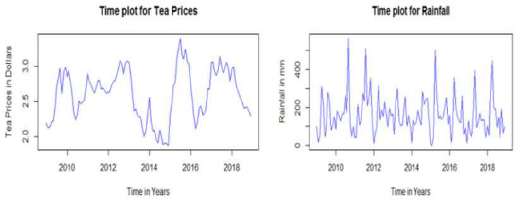 Figure 1Page 4
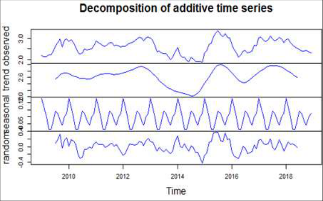 Figure 2Page 4
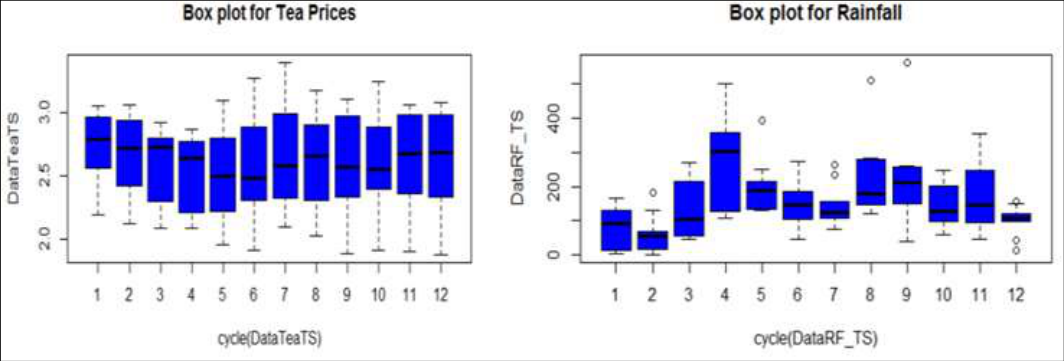 Figure 3Page 5
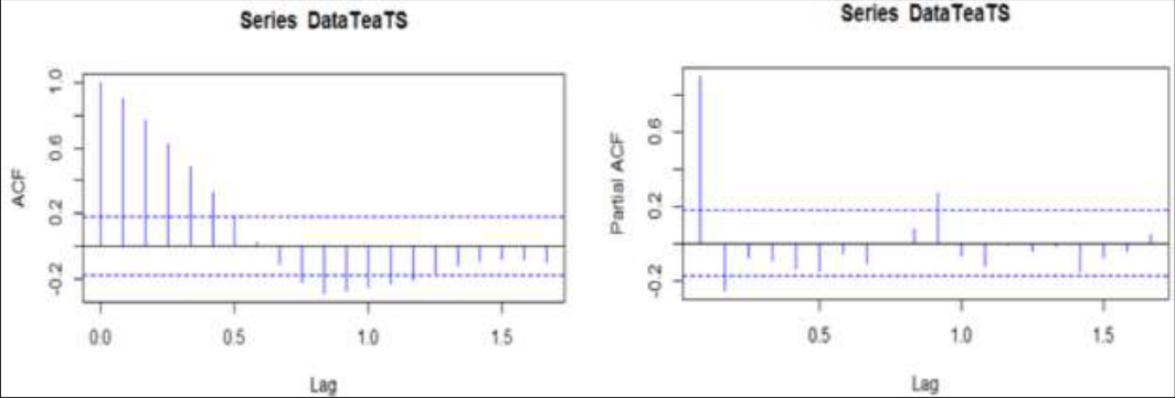 Figure 4Page 5
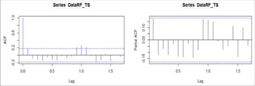 Figure 5Page 5
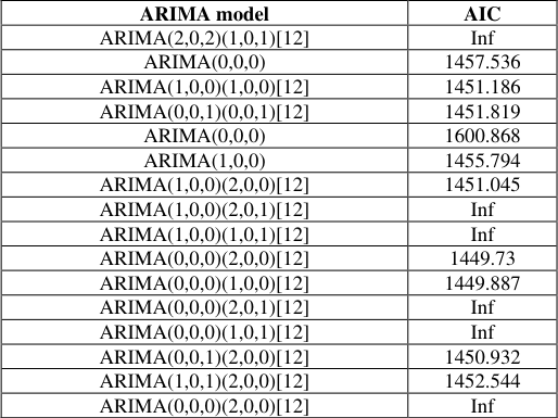 Table 3Page 6
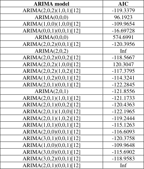 Table 2Page 6
 Table 4Page 6
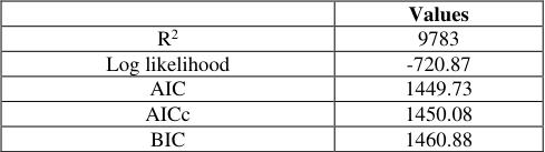 Table 5Page 6
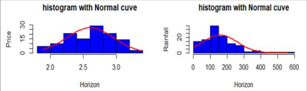 Figure 6Page 6
 Table 6Page 7
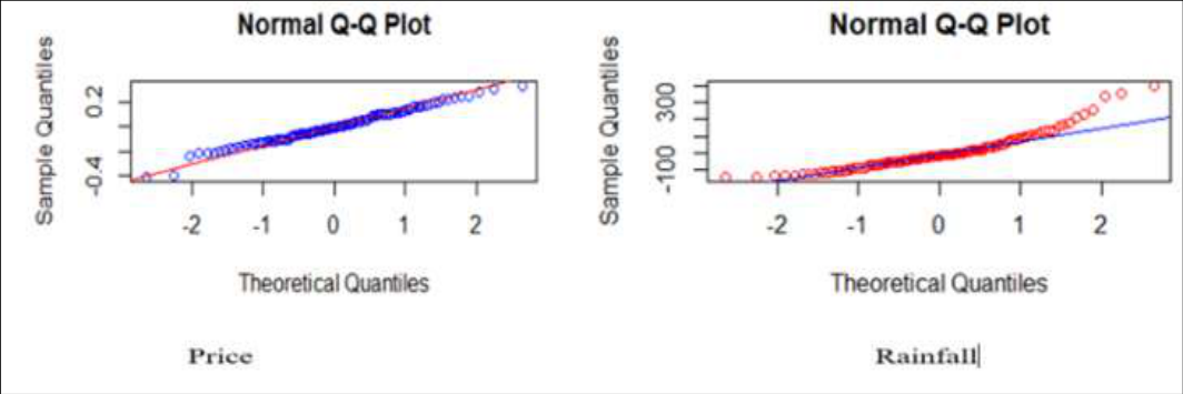 Figure 7Page 7
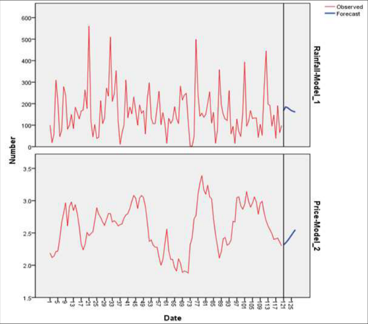 Figure 8Page 7
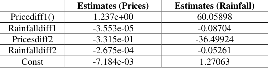 Table 8Page 8
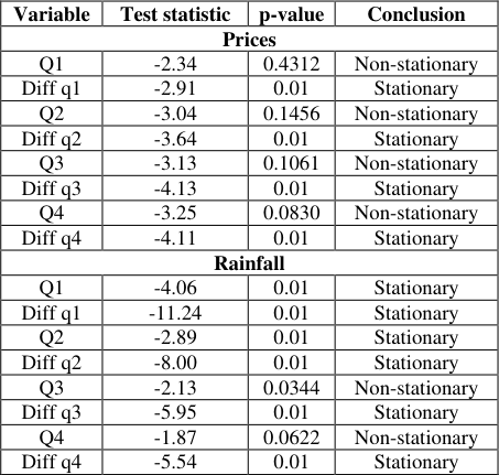 Table 7Page 8
 Table 9Page 8
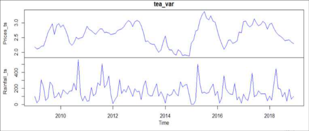 Figure 9Page 8
 Table 11Page 9
 Table 10Page 9
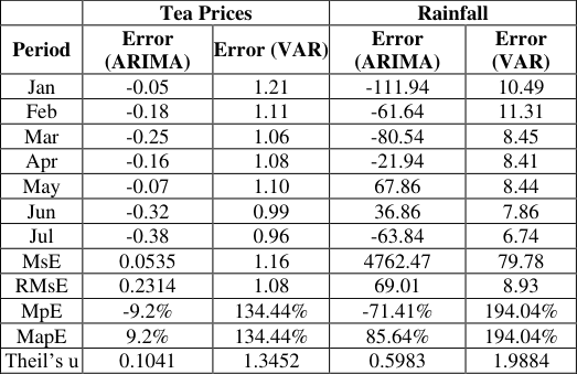 Table 12Page 9
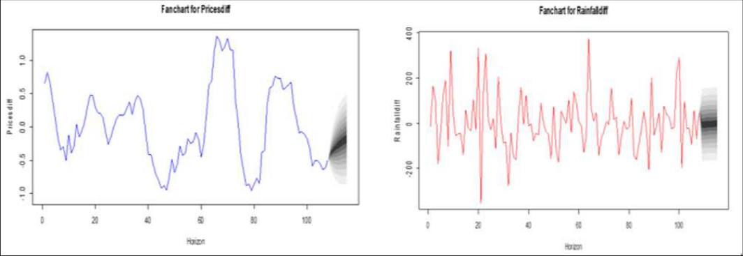 Figure 10Page 9
Introduction
Agriculture has been a major building block in the growth of the economies of most countries around the world. The projections carried out by recent statistics shows that agricultural production needs to increase by 70% by 2050 to meet the growing demand for agricultural products following a report by the International Tea (ITC), 2011.However, availability of cultivable land, inadequate labour, climate change and competition are some of the challenges that affect agricultural production. In Kenya, agriculture plays a vital role in the economic growth and poverty eradication. It is practiced by both small and large scale farmers. Tea is the second most popular beverage in the world after water which has a higher consumption. It is estimated that between 18 and 20 billion 6 oz. cups of tea are drunk daily on our planet. Tea is processed from a plant whose Latin name is: Camellia sinensis. Tea is a very mild stimulant, since it contains caffeine. It contains vitamin A, B2, C, D, K, and P, small quantities of tannic compounds technically called polyphenols, plus a number of minerals in trace amounts and also aromatic oils. The tannin compounds and essential oils are, responsible for the flavor of tea, the color, the dryness, and the delightful aromatics. Global tea production and consumption has tremendously increased in the recent past and is expected to grow further in future both in developing and emerging countries. Accelerated growth has been witnessed by India and China caused by increased demand for the product. Accelerated trend has been contributed by availability of sufficient income and diversification of the product.
China has put more emphasis on specialty items such as fruit fusions, flavored gourmet teas and herbal teas. World tea production has experience a 4.4% annual increase recently. China has been the first tea producer accounting for 42.6% of world tea followed by India. Favorable weather conditions have contributed to this increase. International tea prices have remained firm recently as world tea consumption expanded significantly. Health has been one of the factors contributing to increased consumptions because consumers are now aware of the benefits of this product. Kenya is the largest exporter in black tea followed by China and India; it is projected that these countries will witness an increased production in future according to a report by Food and Agriculture Organization (FAO), 2017 .In this study VAR Model will be used to model and to predict the fitted tea prices incorporating rainfall patterns and then comparing the prediction performance with that of ARIMA model.
Review of Tea Auction Prices Models 2.1 Tea production and prices variability trends
Tea production has increased tremendously in the past few years. The volume of tea produced is constrained by competition e.g. for land, inadequate labor and climate change. According to Agriculture and Food Authority (AFA), 2018 increased production was largely attributed to high rainfall doubled with warm weather conditions experienced in tea growing regions in the west of Rift, majorly; Nyamira, Kisii, Kericho and Nandi. Consequently, output within these regions increased from 29.37 million kilograms in 2017 to 33.26 Million kilograms in 2018. Local tea consumption for 2018 stood at 38.00 million kilograms against 37.63 million kilograms for the corresponding period for 2017. Local consumption has been increasing consistently at an average rate of 5% per annum for the last five years. The value of domestic sales increased consequently from Ksh.15 million in 2017 to Ksh.19 million in the year 2018 attributed by intensive marketing by the government and brand owners. There was an increase of 32% of the total export volume for Kenyan tea in 2018 compared to 2017. The increased production of tea led to overproduction contributed by the high demand for the product which consequently caused the fluctuation of the tea prices. In tea industry, tea prices play a significant role in regulating the economy of its market for the sake of buyers and sellers and also in balancing the supply and demand of the market. Competitiveness of the products is influenced by the prices Kenya is a significant tea producing country in the world and has a great influence on world tea market and also the tea auction market locally.
Review of Generalized Linear Models (GLMs
Hettiarachchi & Banneheka, (2013) [12] . They used Time series regression with Generalized Least Squares and Artificial Neural Network to forecast the seasonally adjusted prices. They performed one-month-ahead forecasts for tea auction prices in Colombo, Kolkata, Cochin, Guwahati, Chittagong, Mombasa and Jakarta. A Box-Cox transformation was used to deal with non-normality. Their results indicated a significant positive correlation between prices at the Colombo auction and those at the other auction centers. Moreover, they compared the forecasting performance of both models and found that the ANN approach performed slightly better than the time series regression approach. However, they were not able to validate their ANN due to the unavailability of weekly tea prices at the auction centers, with the exception of Colombo.
Review of Error Correction Models (ECM)
Dilshani and Chandima (2016) determined whether the using seasonal patterns improved forecasting performance of black tea auction prices with much emphasis on predicting the prices of the Colombo tea auction. Seasonally unadjusted series were tested for seasonal unit roots which provided evidence of presence of common seasonal cycles in monthly black tea auction prices of Colombo, Kolkata and Guwahati centers at six cycles per year. Seasonal co-integration interrelationship was witnessed in the mentioned three tea auction prices which provided the possibility to fit a Seasonal Error Correction Model (SECM). An analysis was carried out for the seasonally adjusted data. It was found that all three seasonally adjusted series were correlated and the series was tested for co-integration interrelationship. Co-integration interrelationship among the series was identified and hence Vector Error Correction (VEC) model was fitted. Adequacy of the fitted SECM and VEC models were tested, and correlograms and unit root tests suggested that the error series were stationary. Using the fitted VEC and SECM models, the future prices was predicted. The accuracy of the forecasts was tested using Mean Absolute Percentage Error (MAPE) and Mean Square Error (MSE). Both measures proved that seasonally unadjusted model gives more accurate predictions than those obtained from the alternative model, during the study period. It was concluded that prediction results are more accurate by taking seasonality into account. However, lack of previous research studies on SECM and adequacy tests had been a challenge faced when carrying out the analysis. This research area is still in the development stage. This research, considered only the tea auction prices of eight major auction centers. Other variables, such as tea production and weather of the major tea export countries should be taken into account to capture the influence from external factors on the tea auction prices. Hewapathirana & Tilakaratne (2012) [11] investigated the behavior of the tea prices of black tea and determined the existence of co-integration among the monthly prices for eight tea auction centres. They used seasonally adjusted data to obtain co-integration among the series and predicted it using Vector Error Correction Model (VECM). Indurawage, Tilakaratne and Rajapaksha (2015), determined whether black tea auction prices with great emphasis on Colombo tea auction in predicting monthly tea auction prices of eight auction centers. Seasonal co-integration interdependence was witnessed which provided the possibility to fit Seasonal Error Correction Model (SECM) and Vector Error Correction (VEC) model. These models were then used to predict the future prices. Performance of the fitted models was then tested using Mean Square Error (MSE) and Mean Absolute Percentage Error (MAPE).
Review of Autoregressive Integrated Moving Average (ARIMA) Model
This model was introduced by Box and Jenkins (1976) [1] which is a merger of autoregressive as well as moving average parameters series. ARIMA modeling takes into account historical data and breaks it down to the Autoregressive process, where there is a series of past events an integrated process which accounts for stabilizing thus making the data easier to forecast; and a Moving Average (MA) of the forecast errors such that the longer the historical data the more accurate the forecasts will be over time. The three components are all combined and interact with each other and recomposed to form the ARIMA (p, d, q) model, where p is the autoregressive parameters, d is the number of differencing phases and q is the moving average parameters. Krishnarani (2013) [8] examined the effect of outlier observations in tea price modeling. Indian tea prices were analyzed using an ARIMA model. Krishnarani's study also searched for the presence of additive and innovational outliers. Krishnarani concluded that the presence of outliers in the price series could be due to variation in climatic variables such as high rainfall, drought and pest outbreaks. Hong Liu and Shuang Shao, (2016) [9] used ARMA model to analyze the sample of India's auction tea prices from 2013 to 2014 obtained weekly. They used the model obtained to forecast the tea price of the last week of 2014 and the first two weeks of 2015. They found that the prediction error was not large. They concluded that a mature tea auction market be established in China, being a major exporter of tea production, and a early warning mechanism for the price of tea should be set so as to guide the production of tea and sales. Price plays a vital role in the market and hence provides a great impact in the regulation of supply and demand. It was recommended that price information mechanism should be improved and a reasonable tea pricing mechanism established. Sneha Chaudhry and Rakesh Kumar Shukla, (2017) [2] carried out a study on time series analysis of auction prices of Indian Tea. The study attempted to identify the variations in Indian tea prices using ARIMA model to study the fluctuations in the tea prices. It found out that there were fluctuations in auction tea prices and major reasons for the fluctuations were identified which contributed to the fluctuating tea prices. N.A.M.R Senaviratna, (2016) analyzed the tea auction prices in Sri Lanka using seasonal ARIMA Model. He found that Seasonal ARIMA(1,0,0)(0,1,0)12 reflected the trend of tea auction prices in Sri Lanka and concluded the models forecast well during and beyond estimation.
Review of Vector Autoregressive (VAR) Model
VAR was introduced by Sims (1980) as a technique used to capture the linear interrelationships among multiple time series. Sims developed the VAR model with lags expressed as VAR (p). Each variable in a VAR model is expressed by an equation explaining its evolution based on its own lagged values. A collection of variables is expressed as a weighted linear combination of the past values in each variable and the past values of the other variables in the collection.VAR (p) models are flexible and easy to use. They are used to describe and forecast stationary multivariate time series.
Methodology 3.1 Study Design and Population
The study used secondary data obtained from the Mombasa Tea auction centre for a period of 2009 to 2018. The data obtained was monthly auction prices and are expressed in US $ per kilogram and rainfall in mm. The study used non cointegration based techniques which are ARIMA and VAR models. The data was applied for description and forecasting of the tea auction prices and rainfall. In most cases univariate time series focuses on a single recognition that is recorded successively over time and in this case ARIMA was applied. The time series data then considered rainfall to obtain the multiple time series data and the VAR model was then applied. Thereafter, it compared the prediction performance results of the two models.
Method of Data Analysis 3.3 Autoregressive Integrated Moving Average (ARIMA) modeling
A non-stationary time series data is made stationary by differencing the series 𝑌 𝑡 . The sequence {𝑌 𝑡 } can be expressed as the general form of ARMA(p, d, q) is,
There are four steps involved in modeling ARIMA include; identification, estimation, diagnostic checking and forecasting.
Model Identification
This refers to initial preprocessing of the data to make it stationary and choosing plausible values of p and q. To identify the p and q components of the ARIMA (p, d, q) model, we plot the sample ACF and PACF of the differenced series to look for behavior that is consistent with stationary processes. The Alkaike Information Criterion (AIC) will be used to evaluate the best model from the set of statistical models. The formula for AIC is; AIC=-2(log-likelihood) + 2K
Where; K is the number of model parameters, log-likelihood is a measure of model fit the higher the number the better the fit.
Parameter estimation
Once a model is identified, the next step of the ARIMA model building process is to estimate the constants (p, d, and q). ARIMA models uses two techniques in the estimation, these are non-linear least squares and maximum likelihood estimation. In this study, parameter estimation was done using a statistical package R.
Model verification
The third step was to check whether the model fits the data. The partial autocorrelation function (PACF) identifies the appropriate lag p in an extended ARIMA (p, d, q) model. Both ACF and PACF were used to check whether the model selected by AIC was appropriate. Two main techniques for model verification are • Over fitting: add extra parameters to the model and use likelihood ratio or t-tests to check that they are not significant. • Residual analysis: calculate residuals from the fitted model and plot their ACF, PACF, 'spectral density estimates', etc, to check that they are consistent with white noise.
Vector Autoregressive (VAR) Modeling
VAR model is used to capture the relationships among multiple time series. It is a generalization of the univariate AR model by allowing more variables that evolve. In order to build a VAR model, (Box and Jenkins, 1976) [1] steps are followed. These include model identification, estimation of the parameters, diagnostic check and finally forecasting.
Model Specification and Identification
When specifying a VAR (p) model, the variables to be included has to be decided. This helps in identifying the order of the appropriate model. The appropriate lag length has to be decided which can be achieved using Akaike Information Criteria (AIC). The smallest possible length has to be chosen. A time series 𝑦 𝑡 , where 𝑦 𝑡 = (𝑦 1𝑡 , 𝑦 2𝑡 , … , 𝑦 𝑛𝑡 ) follows a VAR (p) model if it satisfies;
Parameter estimation
After obtaining the order of the model, p, of the vector series, we now derive the estimators of the parameters. The most common methods of estimating parameters are Maximum Likelihood Estimator (MLE) and Ordinary Least Squares (OLS) estimator. Here, we will apply the Ordinary Least Square (OLS) method. This approach estimates how each independent variable influenced the dependant variable.
Model diagnostic
After a VAR model has been estimated, it is of interest to determine if the residuals obey the assumptions of the model i.e. they are normally, identically and independently distributed .The normal overall checking is a plot of the residuals.
Results and analysis 4.1 Introduction.
This chapter presents the data analysis, presentation of results and discussion of the results. ARIMA and VAR were used to analyze the data, fitted and the fitted models used to predict the future tea auction prices and rainfall. These results are presented and outlined with reference to the objectives of the study.
Auto-Regressive Intergrated Moving Average (ARIMA) Model
This section presents the determination of trend for the tea auction prices in Kenya for a period of 10 years from 2009-2018. The descriptive statistics as shown in the Table 1 below indicate that average price was 2.607 and average rainfall was found to be 158.57mm. The findings based on time series plots as shown in Figure 1 below suggest that the plots are not stationary as evidence by the cyclic and random patterns. The spikes display evidence of strong seasonal variations. Autocorrelation and partial autocorrelation functions were performed in order to transform the non-stationary data into stationary through differencing of the series. Therefore, plots of the series before the first differencing suggests that ARIMA model assumes stationarity with its plot. The ACF and PACF plots before the first difference are shown in Figure 4 and 5 below. The results show that there is little autocorrelation in ACF for both plots of tea prices data and rainfall data. Also, there is no spike closer to one in the PACF plot hence confirming that the data is stationary. Both plots of the series show that there is a little autocorrelation in ACF. Therefore, since the data became stationary before the first order difference, that is at lag 0, then the model that need to be estimated is ARIMA (p, 0, q). Thus, this section aimed at identifying the model, estimating suitable parameters, performing diagnostics for residuals and forecasting auctioning prices of tea. It can be seen that ACF plot for tea prices data decreases gradually after lag 1 while PACF tails off slowly after lag 2 hence the values for p and q for the ARIMA (p, 0, q) model are set at 2 and 1 respectively. Therefore, the ARIMA model to be used for tea prices is ARIMA (2, 0, 1). Moreover, the ACF at lag 1 is significant and positive while PACF cuts off sharply with two significant spikes. Since the plots displays the overall decaying series after few lags, then it indicates a mixed AR (1) and MA (2) model. Also, the ACF plot for rainfall data decreases slowly after lag 1 while PACF died out slowly towards zero. Hence, the values for p and q the ARIMA (p, 0, q) model are set at 0 and 1 respectively and the ARIMA model becomes ARIMA (0, 0, 1). As such, the ARIMA (2, 0, 1) and ARIMA (0, 0, 1) models result to 24 possible combinations for tea prices data as shown in Table 2 below and 16 combinations for rainfall data as shown in Table 3. AIC criteria were used in selecting the most suitable ARIMA model for the series. Taking seasonality into account, the results in Table 2 indicates that the best Seasonal ARIMA model is the ARIMA (2, 0, 1) (0,0,1) [12] with non-zero mean as it has the least AIC value of -122.2845. Also, the best ARIMA Model was found to be ARIMA (2, 0, 1) with the least AIC value -121.8556. ARIMA model AIC ARIMA(2,0,2)(1,0,1) [12] -119.3379 ARIMA(0,0,0) 96.1923 ARIMA(1,0,0)(1,0,0) [12] -109.9654 ARIMA(0,0,1)(0,0,1) [12] -16.69728 ARIMA(0,0,0) 574.6991 ARIMA(2,0,2)(0,0,1) [12] -120.3956 ARIMA(2,0,2) Inf ARIMA(2,0,2)(0,0,2) [12] -118.5667 ARIMA(2,0,2)(1,0,0) [12] 120.3047 ARIMA(2,0,2)(1,0,2) [12] -117.3795 ARIMA(1,0,2)(0,0,1) [12] -114.3241 ARIMA(2,0,1)(0,0,1) [12] -122.2845 ARIMA(2,0,1) -121.8556 ARIMA(2,0,1)(1,0,1) [12] -121.1733 ARIMA(2,0,1)(0,0,2) [12] -120.4363 ARIMA(2,0,1)(1,0,0) [12] -122.1965 ARIMA(2,0,1)(1,0,2) [12] -119.2444 ARIMA(1,0,1)(0,0,1) [12] -115.1263 ARIMA(2,0,0)(0,0,1) [12] -116.6093 ARIMA(3,0,1)(0,0,1) [12] -120.3758 ARIMA(1,0,0)(0,0,1) [12] -109.9648 ARIMA(3,0,0)(0,0,1) [12] -115.6902 ARIMA(3,0,2)(0,0,1) [12] -118.9583 ARIMA(2,0,1)(0,0,1) [12] Inf
| ARIMA model | AIC |
|---|---|
| ARIMA(2,0,2)(1,0,1)[12] | -119.3379 |
| ARIMA(0,0,0) | 96.1923 |
| ARIMA(1,0,0)(1,0,0)[12] | -109.9654 |
| ARIMA(0,0,1)(0,0,1)[12] | -16.69728 |
| ARIMA(0,0,0) | 574.6991 |
| ARIMA(2,0,2)(0,0,1)[12] | -120.3956 |
| ARIMA(2,0,2) | Inf |
| ARIMA(2,0,2)(0,0,2)[12] | -118.5667 |
| ARIMA(2,0,2)(1,0,0)[12] | 120.3047 |
| ARIMA(2,0,2)(1,0,2)[12] | -117.3795 |
| ARIMA(1,0,2)(0,0,1)[12] | -114.3241 |
| ARIMA(2,0,1)(0,0,1)[12] | -122.2845 |
| ARIMA(2,0,1) | -121.8556 |
| ARIMA(2,0,1)(1,0,1)[12] | -121.1733 |
| ARIMA(2,0,1)(0,0,2)[12] | -120.4363 |
| ARIMA(2,0,1)(1,0,0)[12] | -122.1965 |
| ARIMA(2,0,1)(1,0,2)[12] | -119.2444 |
| ARIMA(1,0,1)(0,0,1)[12] | -115.1263 |
| ARIMA(2,0,0)(0,0,1)[12] | -116.6093 |
| ARIMA(3,0,1)(0,0,1)[12] | -120.3758 |
| ARIMA(1,0,0)(0,0,1)[12] | -109.9648 |
| ARIMA(3,0,0)(0,0,1)[12] | -115.6902 |
| ARIMA(3,0,2)(0,0,1)[12] | -118.9583 |
| ARIMA(2,0,1)(0,0,1)[12] | Inf |
Table text extracted from the original PDF; superscript letters are shown inline. The original table image is below.
View original table image
| ARIMA model | AIC |
|---|---|
| ARIMA(2,0,2)(1,0,1)[12] | Inf |
| ARIMA(0,0,0) | 1457.536 |
| ARIMA(1,0,0)(1,0,0)[12] | 1451.186 |
| ARIMA(0,0,1)(0,0,1)[12] | 1451.819 |
| ARIMA(0,0,0) | 1600.868 |
| ARIMA(1,0,0) | 1455.794 |
| ARIMA(1,0,0)(2,0,0)[12] | 1451.045 |
| ARIMA(1,0,0)(2,0,1)[12] | Inf |
| ARIMA(1,0,0)(1,0,1)[12] | Inf |
| ARIMA(0,0,0)(2,0,0)[12] | 1449.73 |
| ARIMA(0,0,0)(1,0,0)[12] | 1449.887 |
| ARIMA(0,0,0)(2,0,1)[12] | Inf |
| ARIMA(0,0,0)(1,0,1)[12] | Inf |
| ARIMA(0,0,1)(2,0,0)[12] | 1450.932 |
| ARIMA(1,0,1)(2,0,0)[12] | 1452.544 |
| ARIMA(0,0,0)(2,0,0)[12] | Inf |
Table text extracted from the original PDF; superscript letters are shown inline. The original table image is below.
View original table image
| — | Min | Median | Mean | Max |
|---|---|---|---|---|
| Price | 1.880 | 2.660 | 2.607 | 3.390 |
| Rainfall | 2.30 | 134.25 | 158.57 | 560.80 |
Table text extracted from the original PDF; superscript letters are shown inline. The original table image is below.
View original table image
In addition, the results in Table 3 suggest that the best Seasonal ARIMA Model was found to be ARIMA (0,0,0)(2,0,0) [12] with the least AIC value of 1449.73 while ARIMA (1, 0, 0) was found to be the best ARIMA model for the rainfall data. ARIMA model AIC ARIMA(2,0,2)(1,0,1) [12] Inf ARIMA(0,0,0) 1457.536 ARIMA(1,0,0)(1,0,0) [12] 1451.186 ARIMA(0,0,1)(0,0,1) [12] 1451.819 ARIMA(0,0,0) 1600.868 ARIMA(1,0,0) 1455.794 ARIMA(1,0,0)(2,0,0) [12] 1451.045 ARIMA(1,0,0)(2,0,1) [12] Inf ARIMA(1,0,0)(1,0,1) [12] Inf ARIMA(0,0,0)(2,0,0) [12] 1449.73 ARIMA(0,0,0)(1,0,0) [12] 1449.887 ARIMA(0,0,0)(2,0,1) [12] Inf ARIMA(0,0,0)(1,0,1) [12] Inf ARIMA(0,0,1)(2,0,0) [12] 1450.932 ARIMA(1,0,1)(2,0,0) [12] 1452.544 ARIMA(0,0,0)(2,0,0) [12] Inf
Parameter Estimation.
After identification of the model, it was evidenced that ARIMA (2, 0, 1)(1, 0, 0) was the best model the estimated parameters and model fits are shown in Table 4 and 5 below. Model diagnostics tests were performed to check whether the fitted model is significant. The plot frequency distribution of the residuals as shown in Figure 6 below of the fitted model ARIMA (2, 0, 1×0, 0, 1) indicates the residuals for price is normally distributed while for rainfall is fairly normal. The QQ-plots as shown in Figure 7 suggests that the plot for tea prices has no outliers and all points lie on the line while the plot for rainfall has some few outliers though not significant. Therefore, the residuals of the fitted model are normally distributed. Furthermore, the p-values of the Ljung box test as shown in Table 6 below are greater than 0.05 hence suggesting that the fitted Seasonal ARIMA (2,0,1)(0,0,1) model is the best fitted model. The fitted Seasonal ARIMA model is used to forecast tea prices and rainfall for the year 2019 and comparing them with the observed values. The results as presented in Table 7 for below suggest that the forecasted values are relatively close to the observed values. Also, the forecast for 2019 is shown in Figure 8 below.
| Variable | Test statistic | p-value | Conclusion |
|---|---|---|---|
| Prices | |||
| Q1 | -2.34 | 0.4312 | Non-stationary |
| Diff q1 | -2.91 | 0.01 | Stationary |
| Q2 | -3.04 | 0.1456 | Non-stationary |
| Diff q2 | -3.64 | 0.01 | Stationary |
| Q3 | -3.13 | 0.1061 | Non-stationary |
| Diff q3 | -4.13 | 0.01 | Stationary |
| Q4 | -3.25 | 0.0830 | Non-stationary |
| Diff q4 | -4.11 | 0.01 | Stationary |
| Rainfall | |||
| Q1 | -4.06 | 0.01 | Stationary |
| Diff q1 | -11.24 | 0.01 | Stationary |
| Q2 | -2.89 | 0.01 | Stationary |
| Diff q2 | -8.00 | 0.01 | Stationary |
| Q3 | -2.13 | 0.0344 | Non-stationary |
| Diff q3 | -5.95 | 0.01 | Stationary |
| Q4 | -1.87 | 0.0622 | Non-stationary |
| Diff q4 | -5.54 | 0.01 | Stationary |
Table text extracted from the original PDF; superscript letters are shown inline. The original table image is below.
View original table image
| — | Chis-value | Df | p-value |
|---|---|---|---|
| Price | 22.527 | 15 | 0.095 |
| Rainfall | 23.587 | 15 | 0.073 |
Table text extracted from the original PDF; superscript letters are shown inline. The original table image is below.
View original table image
| Coefficients | Estimates | Standard errors |
|---|---|---|
| sar1 | 0.2443 | 0.0940 |
| sar2 | 0.1533 | 0.1033 |
| mean | 157.4211 | 13.6158 |
Table text extracted from the original PDF; superscript letters are shown inline. The original table image is below.
View original table image
Testing Stationarity.
Augmented dickey-fuller(ADF) test was performed on the series in order to check for stationarity of the data by testing the unit roots. The results as shown in Table 8 below suggest that all the variables are not stationary since there p-values are greater than 0.01. First differencing of the series resulted to stationarity of the variables hence all the time series were integrated of at least order one.
| — | Estimates (Prices) | Estimates (Rainfall) |
|---|---|---|
| Pricediff1() | 1.237e+00 | 60.05898 |
| Rainfalldiff1 | -3.553e-05 | -0.08704 |
| Pricesdiff2 | -3.315e-01 | -36.49924 |
| Rainfalldiff2 | -2.675e-04 | -0.05261 |
| Const | -7.184e-03 | 1.27063 |
Table text extracted from the original PDF; superscript letters are shown inline. The original table image is below.
View original table image
Model diagnostic.
First, the fitted model was tested for autocorrelation using Box Ljung tests for checking whether the residuals are identically distributed. The results as shown in Table 10 below suggest that the p-value for tea prices was less than 0.01 hence this show that tea prices depicted some sign of autocorrelation thus has inconsistent estimators. However, the p-value for rainfall was greater than 0.01 hence rainfall show some signs of no autocorrelation thus has consistent estimators. Second, the fitted model was tested for the presence of heteroskedasticity using arch tests. The results as shown in Table 11 below suggest that there was no presence of heteroscedasticity in the model or no auto effects correlation were observed in the model as the p-value was found to be
| — | Chi-sq | p-values |
|---|---|---|
| JB test | 10.883 | 0.02791 |
| Skewness | 3.2422 | 0.1977 |
| Kurtosis | 7.6408 | 0.02192 |
Table text extracted from the original PDF; superscript letters are shown inline. The original table image is below.
View original table image
Conclusions
Tea plays a significant role in the economies of most tea producing countries. Kenyan tea has a great impact on the world tea market and auction system locally. However, tea industry in Kenya has gone through many phases of ups and downs in terms of its export performance. Therefore there was need to carry out a study on tea prices in order to accord it a competitive part in the global market. This study therefore aimed at predicting the behavior of tea auction prices where rainfall pattern was incorporated in the series. The results suggested Seasonal ARIMA (2, 0, 1)(0,0,1) model to be appropriate for modelling tea prices as compared to VAR (2) model. Therefore, this model can be applied by tea planters and policy makers in making appropriate decisions regarding pricing trends in Tea industry.
Recommendations
The study considered the trend of tea auction prices in Kenya, it is important for further research to include trends of tea auction prices from other auction centers. There is need to consider other variables such as tea production and climate factors, e.g temperature as a factor of climate is incorporated in the modelling trends of tea auction prices so as to determine the effect of external factors on tea auction prices in other major auction centers. Further research also should consider use of seasonally unadjusted series in fitting Nonliear Autoregressive network with Exogenous input for forecasting tea auction prices. In addition, price plays a vital role in the market and hence provides a great impact in the regulation of tea supply and demand. Therefore, price information mechanism should be improved and a reasonable tea pricing mechanism be established.
Figures and tables from the paper
| — | Values |
|---|---|
| R2 | 9783 |
| Log likelihood | -720.87 |
| AIC | 1449.73 |
| AICc | 1450.08 |
| BIC | 1460.88 |
Table text extracted from the original PDF; superscript letters are shown inline. The original table image is below.
View original table image
| — | Tea Prices | — | Rainfall | — |
|---|---|---|---|---|
| Period | Error (ARIMA) | Error (VAR) | Error (ARIMA) | Error (VAR) |
| Jan | -0.05 | 1.21 | -111.94 | 10.49 |
| Feb | -0.18 | 1.11 | -61.64 | 11.31 |
| Mar | -0.25 | 1.06 | -80.54 | 8.45 |
| Apr | -0.16 | 1.08 | -21.94 | 8.41 |
| May | -0.07 | 1.10 | 67.86 | 8.44 |
| Jun | -0.32 | 0.99 | 36.86 | 7.86 |
| Jul | -0.38 | 0.96 | -63.84 | 6.74 |
| MsE | 0.0535 | 1.16 | 4762.47 | 79.78 |
| RMsE | 0.2314 | 1.08 | 69.01 | 8.93 |
| MpE | -9.2% | 134.44% | -71.41% | 194.04% |
| MapE | 9.2% | 134.44% | 85.64% | 194.04% |
| Theil’s u | 0.1041 | 1.3452 | 0.5983 | 1.9884 |
Table text extracted from the original PDF; superscript letters are shown inline. The original table image is below.
View original table image
References
9 in the original paper- Box GE, Jenkins GM. Time Series Analysis: Forecasting and Control san Francisco. Calif: Holden-Day 1976.
- Dharmasena KASDB. International black tea market integration and price discovery (PHD thesis), Texas A & M University 2004.
- Hettiarachchi H, Banneheka B. Time Series Regression and Artificial neural network approaches for forecasting unit price of tea at Colombo auction. Journal of the national science foundation of Sri Lanka, 2012, 41(1).
- Krishnarani SD. Time series outlier analysis of tea price data American Journal of Theoretical and Applied Statistics 2013;2(1):1-6.
- Liu H, Shao S. India's Tea Price Analysis Based on ARMA Model. Modern Economy 2016;7(2):118-123.
- Zivot E, Wang J. Unit root tests. Modelling Financial Time Series with S-PLUS, Springer, pages 2006, 111139.
- Hewapathirana IU, Tilakaratne CD. Modeling and Forecasting Sri Lankan black tea prices exploring temporal patterns, Proceedings of the ISM International Statistical Conference 2012, Johor Bharu, Malaysia 2012.
- Hettiarachchi HACK, Banneheka BMSG. Time Series Regression and Artificial Neural Network Approaches for Forecasting Unit Price of Tea at Colombo Auction. Journal of the National Science Foundation Sri Lanka 2012;41:35-40.
- Dharmasena KASDB, Bessler DA. Weak Form Efficiency Vs Semi Strong Form Efficiency in Price Discovery: An Application to International Black Tea Markets, Sri Lankan Journal of Agricultural Economics 2004;6(1):2004.