
Research article · 2021 · Full text
International Journal of Statistics and Applied MathematicsTransforming demand function to linear function
Volume 6(2) · Pages 31–36 · DOI: 10.22271/maths.2021.v6.i2a.661 ↗
Research areasAgricultural Economics and PracticesOptimization and Mathematical Programming
Abstract
Author-writtenThe research aimed to transform the nonlinear demand function to linear function using statistical and mathematical models by using logarithms and dummy variables. The research resulted in that the linear model is a good alternative for nonlinear model.
Summary
Source-checkedPlain-language reading of the full paper, prepared with AI and checked against the text. Each point links to the authors' own words.
Why it matters
- Demand is defined as a consumer's desire to purchase a commodity or service and their willingness to pay for it. View evidence ↗
- There is an inverse relationship between price and demand, meaning that as the price of a commodity or service increases, the demand for it decreases. View evidence ↗
- The demand curve, which describes demand as a function of price, is typically represented by a nonlinear function. View evidence ↗
The question
- The research aims to transform a nonlinear demand function into a linear function using logarithms, dummy variables, and mathematical models. View evidence ↗
- The goal is to enable the estimation of demand for multiple commodities or services using ordinary least squares (OLS) by linearizing the function. View evidence ↗
What they did
- The first step of the transformation involves applying logarithms to both sides of the nonlinear demand equation. View evidence ↗
- Dummy variables are introduced to capture parameter valuation, as least square models require a constant parameter for estimation. View evidence ↗
- The ordinary least square (OLS) method is applied to estimate the parameters of the resulting linear model. View evidence ↗
- The models were tested using 20 months of data on the demand (in packages) and price (in thousand Sudanese pounds) for dates in the Atbara market. View evidence ↗
What they found
- The estimated linear model was found to be highly significant, with a P-value of 0 and an R-squared value of 63.5%. View evidence ↗
- Price, the independent variable in the model, was determined to be highly significant with a P-value of 0. View evidence ↗
- The constant term was not significant, which the authors state is logical because demand is zero when the price is zero. View evidence ↗
- The price coefficient was negative, supporting the expected inverse relationship between demand and price. View evidence ↗
- Comparison of the predicted values from the original nonlinear model and the transformed linear model showed they are approximately equal. View evidence ↗
What it means
- The authors conclude that the linear model serves as a good alternative to the nonlinear model for demand functions. View evidence ↗
- The study concludes that the transformed linear model (equation 17) can be used as an alternative to the original nonlinear model (equation 1). View evidence ↗
Visual summary
1 visualsIllustrations explain the paper; they do not show study data.
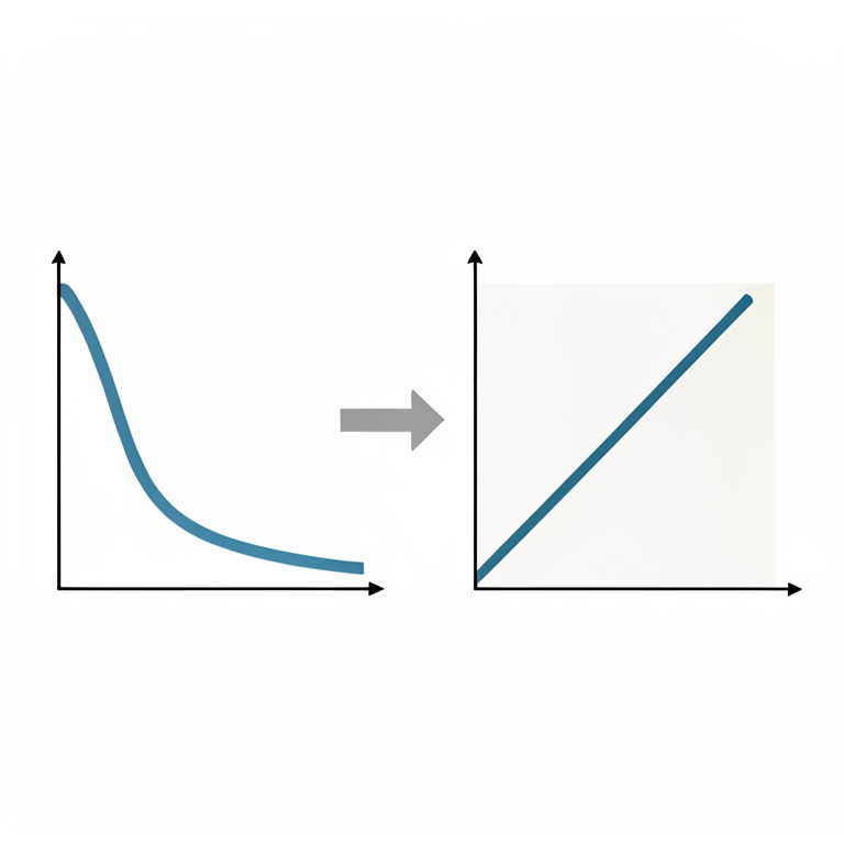
Nonlinear to Linear Transformation
AI-generated conceptual illustration (A mathematical coordinate plane with geometric lines). It explains the idea and does not show study data.
View source evidence ↗Figures & tables
From the original paper Table 1
 Table 1
 Table 2
 Table 3
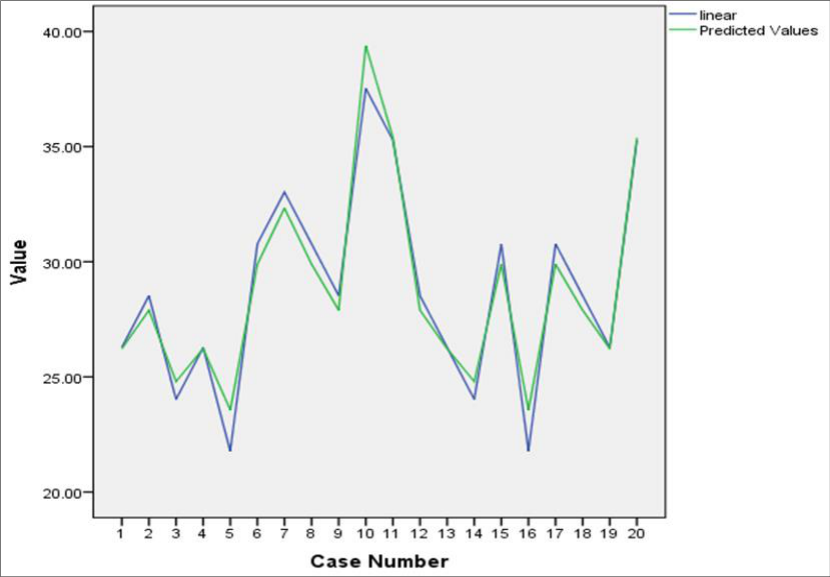 Figure 1
Introduction
Demand for any commodity or services referring to a consumer's desire to purchase and willingness to pay a price for it. And it has an inverse relationship with price i.e., increasing in price of any commodity or service decreases the demand for it and vice versa. And the graph for demand and price which is called demand curve has a nonlinear function that describes the demand as a function of price as follows [3]. μ P α D it b it i it .., N. , , , i = = 3 2 1 .,T , , , t = 3 2 1 (1) Where: Dit: Is the quantity demanded from commodity i at time period t. Pit: Is the price of commodity i at time t.
Uit: Is the error term for commodity i at time period t, with the following assumptions: E = 0 it 2 2 E = ( ) ( ) it = = = 0 ( ) ( ) ( ) s t and j i for E E E js it jt it is it i : Is the intercept term, and the index "i " indicate that the intercepts are differ from commodity to another. b: Is the slope coefficient, and it represents the elasticity of demand, which is defined as the relative change in the quantity demanded (ΔD) divided by the relative change in the price(Δ) , i.e. P D b = Maths 2021; 6(2): 31-36 Abdallah Ahmed Alkhalifa Department of Statistics, Tabuk Faculty of Science University (KSA), Saudi Arabia Abdallah Ahmed Alkhalifa Department of Statistics, Tabuk Faculty of Science University (KSA), Saudi Arabia http://www.mathsjournal.com The aim of this paper is to transform nonlinear demand function to linear function, - butting in consideration that data is available for many commodities or services - so that it can be estimated by using ordinary least squares (OLS).
Methods
and procedures First, introducing log to the two sides of equation (1): [3] log log it it i it P b Log D Log + + = (2) When estimating this equation, it's useful to leave it in its log form than to translate it back into exponential form, because change in (say log'x') is approximately equal to the relative change in (x) itself. This result follows from the elementary differentiation formula: x Log ( ) = 1 x x = x x Log ( ) x i.e., change in log(x) = relative change in (x) Now, let: X P Log Y D Log = = it it it it e Log a Log = = ( ) ( ) ( ) ( ) it it i i (3) Substituting equation (3) into equation (2) we obtain: it it i it e bX a Y + + = (4) Second, Introducing Dummy Variables to capture valuation in parameters comes from that using least square or generalized least square models must have a constant parameter to be estimated and then using least square or generalized least square is not clear what they are estimators of therefore:[2] Now equation (4) can be written as: N it it j j it e bX D a Y + + = j 1 = (5) Where it D is the dummy variable and defend as: j j if D jt 1 0 = = i j if Equation (5) can be written as: N e bX D a D a Y + + + = it it jt j j t it 2 1 1 = N + = + + + + = a a e bX D a D a , ( ) j j it it jt j 1 1 2 1 1 j t = N N + + + = e bX D D a jt it it jt j 2 1 1 j = = j N N + + + = e bX D a = 1 it it jt j jt D 2 1 j = j = 1 (6) http://www.mathsjournal.com [The last step obtained by taking the constraint Third, estimating the parameters:[4] We can write equation (5) as follows: N it it jt j it e bX D a Y + + = j =1 In matrix notation as: + + = e b X j a Y i i T j i ,........, 1 N i = (7) Where: = iT i i i Y Y Y Y . ,......... , ,2 1 Tj 1 ... ,......... 1,1 ) 1 (T = = iT i i i X X X X ... .......... 2 1 = iT i i i e e e e ....... .......... 2 1 Or in more compact form as: a 1 e Y X 0 1 1 T a 1 2 Y X e J J 2 2 2 T = + or a Y X 0 J = N e N N N T b e b a X J I Y T N + (8) Now equation (8) takes the form of the general linear mode: e X Y + = (9) Where, Y Y Y Y = ....... 2 1 N X J I X = T N a − = b e e e e = . .......... N 2 1 Then, Appling ordinary least square method to estimates : ˆ ( ) Y X X X = −1 ˆ http://www.mathsjournal.com −1 = / ˆ ˆ J I b a ie T N T N T N ( ) ( ) Y X = J I X J I X − 1 ( ) Y J I ( ) T N IN X J I T T N = X X J I X Y X ( ) T N (10) But if N is large the inversion of X in equation (9) will be unreliable, so an alternative expression is suggested for estimating "a " and "b": [2] ( )( ) ) ( ) ] [ ˆ 1 Y D I X X D I X b T N T N = − (11) Where: − = J J I D T T T T T and ˆ . ˆ .b X i Y a i i − = where : t T . 1 . , 1 = = it it i X T i X Y T Y t = = 1 1 t (These alternative expressions are obtained from equation (10) by using the partition inverse) And to simplify the computation procedure in practice, it can be shown that DT is idempotent and hence ( T N D I ) is also idempotent. Therefore, equation (11) can be written as: − − ( ) 1 w Z Z Z = ( ( ) ( ) ) ( ) ( ) ˆ 1 Y D I D I X X D I D I X b T N T N T N T N = (12) Where: ( ) X D I Z T N = (13) ( ) Y D I w T N = (14) Then, transform the observation on the independent variable and the dependent variable as follows: equation (13) will be: X X D O D 1 T 1 T X X D D 2 T 2 T = = = ( ) T N X D I Z D O X X D N T N T Examining the ith vector: T i i T T T i T J i X X X T J J I X D . − = − = http://www.mathsjournal.com X J = .i i T X T Since * . it i it it T X X X X D = − = (15) And similarly, equation (14) will be: Y D I w = ( ) T N Y Y Y Y D = − = . it i it it T (16) Now the transformed model is: where .i it it it it it e e e e b X Y − = + = (17) Then the generalized least square estimate for b is: ( ) ˆ 1 − = Y X X X b (18) The linear model in (17) has no intercept, because if price is zero there is no demand. Comparing results between the two models Appling equation (1) and equation (18) to the following data which show demand (in Packages) and price (in thousand Sudanese pounds) for dates in Atbara market for 20 months: demand 20 25 23 24 21 32 35 33 31 36 38 27 29 28 25 24 28 27 26 33 price 10 9 11 10 12 8 7 8 9 5 6 9 10 11 8 12 8 9 10 6 Applying equation (1) results in significant model, then applied the alternative model of equation (18) we get the following
Results
Table 1: Model Summaryb Model R R Square Adjusted R Square Std. Error of the Estimate 1 .797a .635 .615 3.40333 a. Predictors: (Constant), p b. Dependent Variable: d Table 2: ANOVAa Model Sum of Squares df Mean Square F Sig. 1 Regression 363.263 1 363.263 31.363 .000b Residual 208.487 18 11.583 Total 571.750 19 a.
| Model | — | Sum of Squares | df | Mean Square | F | Sig. |
|---|---|---|---|---|---|---|
| 1 | Regression | 363.263 | 1 | 363.263 | 31.363 | .000b |
| Residual | 208.487 | 18 | 11.583 | |||
| Total | 571.750 | 19 | ||||
| a. Dependent Variable: d | ||||||
| b. Predictors: (Constant), p |
Table text extracted from the original PDF; superscript letters are shown inline. The original table image is below.
View original table image
Dependent Variable: d b. Predictors: (Constant), p Table 3: Coefficientsa Model Unstandardized Coefficients Standardized Coefficients t Sig. B Std. Error Beta 1 (Constant) -7.991E-16 .761 .000 1.000 p -2.249 .402 -.797 -5.600 .000 a.
| Model | — | Unstandardized Coefficients | — | Standardized Coefficients | t | Sig. |
|---|---|---|---|---|---|---|
| B | Std. Error | Beta | ||||
| 1 | (Constant) | -7.991E-16 | .761 | .000 | 1.000 | |
| p | -2.249 | .402 | -.797 | -5.600 | .000 | |
| a. Dependent Variable: d |
Table text extracted from the original PDF; superscript letters are shown inline. The original table image is below.
View original table image
Dependent Variable: d The above results shows that the model is highly significant with P-value = 0 in the ANOVA table and R2 =63.5% and in the estimated model the price (independent variable) is highly significant (P-value = 0) while the constant is not significant because if price is zero there is no demand which is logical result. Also, Price coefficient is negative which support the inverse relationship between demand and price. http://www.mathsjournal.com Fig 1: Graphing predicted values for both models we get: Which indicate that the predicted values for two models are approximately equal.
Conclusion
From the results obtained in this study, we can conclude that the model of equation (17) can be alternative for the model of equation (1).
References
4 in the original paper- Judge Hill, Griffths Lee. Introduction to the theory and practice of econometrics, second edition, John willy & sons 1988.
- Koutsoyannis A. Theory of econometrics, second edition 1977.
- Terry Dielman E. Pooled cross sectional and time series data analysis 1989.
- Wallace TD, Ashiq Hussain. The use of error components models in combining cross section with time series data, econometrica 1969;37:55-71.