
Research article · 2021 · Full text
International Journal of Statistics and Applied MathematicsDesign and development of intra lot group acceptance chain sampling plans with an emphasis on zero tolerance non-conformities
Volume 6(1) · Pages 100–106
Research areasAdvanced Statistical Process MonitoringOptimal Experimental Design Methods
Abstract
Author-writtenIn this article a new sampling plan to control product quality known to be Intra Lot Group Acceptance Chain Sampling Plan (ILGAChSP) is developed. Group Acceptance Sampling Plans are widely used in life testing experiments and has applications in research and development centers. In many testing fields, zero defective is expected in every groups or batches. Hence in this paper zero defective is emphasized during testing with an allowance of a non-conformity in a chain of i groups within the same batch of products. If a defective is found then the batch will be accepted only if ‘i’ consecutive chain of groups have zero defective in the current lot. Since ‘i’ chain of groups are tested in the same batch or lot it is termed as Intra Lot Group Acceptance Chain Sampling Plans.
Summary
Source-checkedPlain-language reading of the full paper, prepared with AI and checked against the text. Each point links to the authors' own words.
Why it matters
- Acceptance sampling tools are critical components of quality control in modern industrial settings. View evidence ↗
- Group acceptance sampling plans are beneficial because they can reduce inspection costs and testing time by testing more items simultaneously. View evidence ↗
- In life testing experiments, there is often a requirement for zero tolerance regarding non-conformities within each group. View evidence ↗
The question
- The authors aim to develop a novel Intra Lot Group Acceptance Chain Sampling Plan (ILGAChSP) to address existing gaps in quality control for single lots. View evidence ↗
What they did
- The method involves drawing a random sample of size n (where n = g * r), dividing them into 'g' groups with 'r' items per group for life testing. View evidence ↗
- A lot is accepted immediately if zero non-conformities are found across all groups in the first sample. View evidence ↗
- The lot is rejected if more than one non-conformity is found in the first sample. View evidence ↗
What they found
- The ILGAChSP is effective at discriminating between high-quality (good) and low-quality (bad) lots. View evidence ↗
- The Operating Characteristic (OC) curve exhibits a 'good shoulder effect,' providing confidence to producers that quality is being maintained. View evidence ↗
- The outgoing quality of a batch after inspection is lower than the incoming quality, which is an advantage for the consumer. View evidence ↗
- Increasing the chaining index 'i' leads to a decrease in the operating ratio. View evidence ↗
What it means
- The authors conclude that the developed tables enable quality control practitioners to implement the ILGAChSP in practice. View evidence ↗
- The authors state that the probability of lot acceptance drops rapidly as product quality deteriorates. View evidence ↗
Visual summary
3 visualsIllustrations explain the paper; charts are replotted from the paper's own table values.
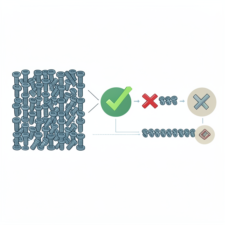
ILGAChSP Decision Flowchart
AI-generated conceptual illustration (industrial mechanical components in a quality control setting). It explains the idea and does not show study data.
View source evidence ↗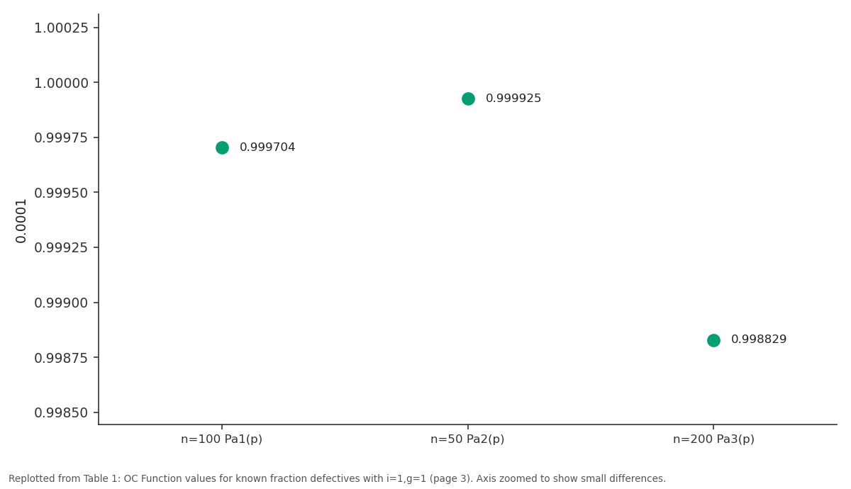
0.0001: n=100 Pa1(p) vs n=50 Pa2(p) vs n=200 Pa3(p)
Replotted from Table 1 (page 3) of the original paper. Every bar is the paper's own table value.
View source evidence ↗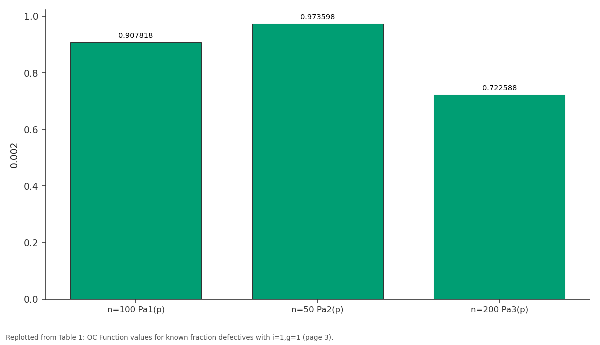
0.002: n=100 Pa1(p) vs n=50 Pa2(p) vs n=200 Pa3(p)
Replotted from Table 1 (page 3) of the original paper. Every bar is the paper's own table value.
View source evidence ↗Figures & tables
From the original paper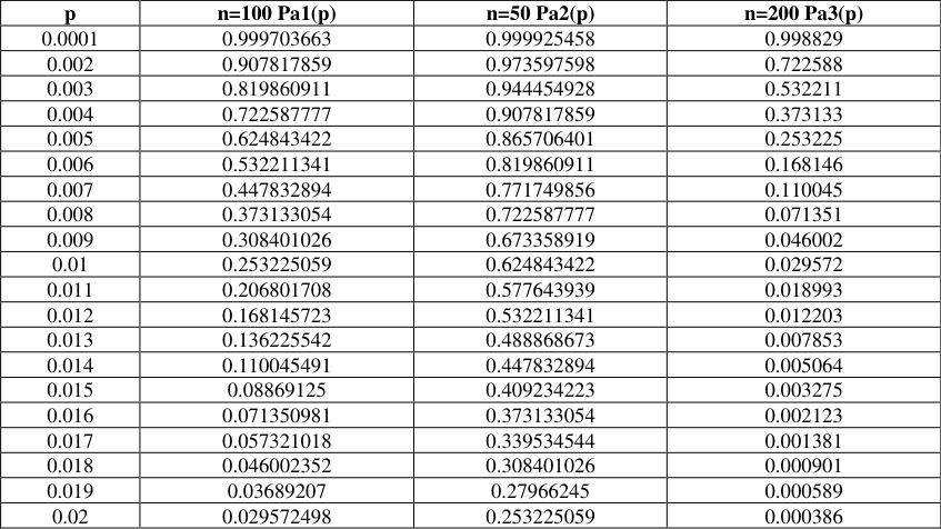 Table 1
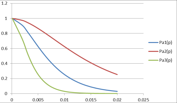 Figure 1
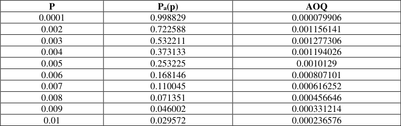 Table 2
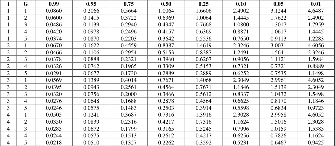 Table 3
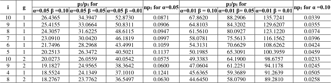 Table 4
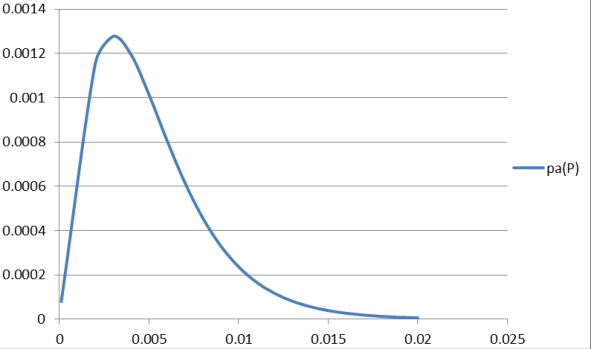 Figure 2
 Table 5
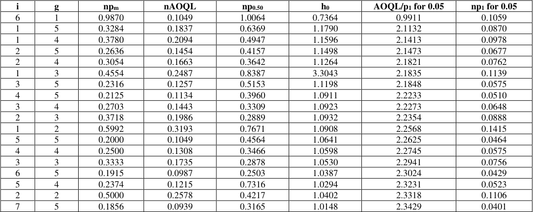 Table 5
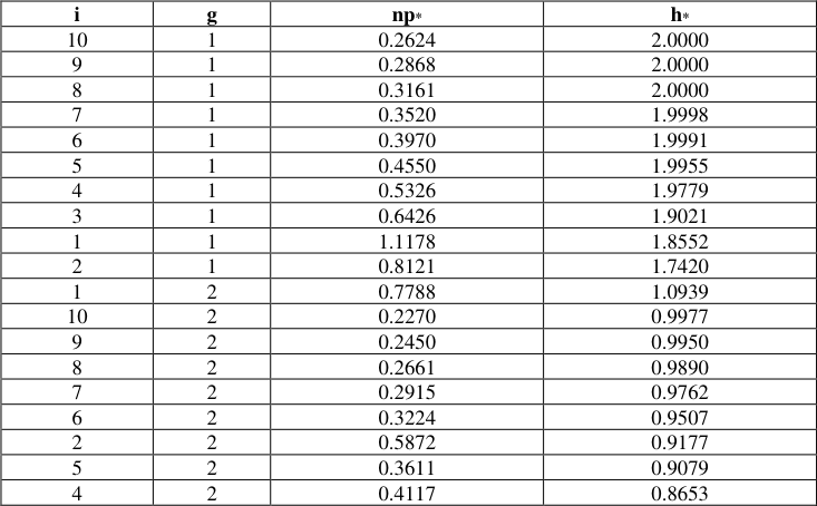 Table 6
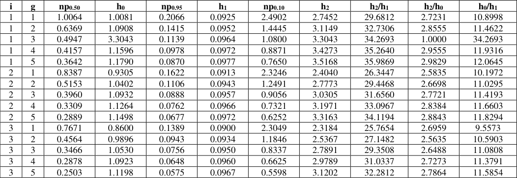 Table 7
Introduction
In modern industries acceptance sampling tools and techniques are one of the major components in the field of quality control division. These techniques are employed for incoming or receiving lots of the quality of the product manufactured in the industries. The advantage of group acceptance sampling plans is it saves the testing time and reduces the cost of inspection if more items are tested in an experiment. Dodge (1955) [9] has found that zero acceptance numbers in certain sampling plans does not discriminate between good and bad lots. Hence he suggested an allowance of one defective in the current lot and with zero defective in the preceding i lots. But in modern industries quality control practitioners insist that when the sampling plan is administered then the first lot should be capable of meeting the consumer requirement. In fact during life testing experiment they need zero tolerance non conformities in each group. If a defective is found then the same experiment is to be conducted for i such groups in the same lot and the lot should be accepted if all the successive chain of groups have zero defective during testing. Hence in order fulfill the need and lacunae, a novel Intra Lot Group Acceptance Chain Sampling Plans are developed. The efficiency measures Operating Characteristic Function, ASN, ATI, AOQ are developed. Designing through standard quality levels leads to the determination of parameters. The motto of this article is to improve the efficiency of sampling algorithm of the Group Acceptance Sampling with Chain sampling procedure for a single lot. Srinivasa Rao G, et al. (2020), have developed Group Acceptance Sampling Plans for Resubmitted Lots under Type II Generalized Half Logistic Distribution. "Resubmitted sampling plan consists of repeat sampling process, once the consumer is not accepted a production lot based on a single acceptance sampling plan then take the second sample of same size for testing; and build a decision removing the first sample results under the provisions of the statutes or contract". Muhammad Aslam and Chi-Hyuck Jun (2009) [15] , have contributed to GASP for truncated life tests based on the inverse Rayleigh and Log-Logistic distributions. They have compared the results for the two distributions, the inverse Rayleigh and loglogistic distributions when the consumer's risk and the other plan parameters are specified. The minimum number of groups required is determined by considering the consumer's risk when the true mean equals the specified life (μ = μ 0 ). Srinivasa Rao G (2009) [32] , has studied GASP for generalized exponential distribution. The number of groups g required for in the case of the generalized exponential distribution is determined. Muhammad Aslam, et al., (2017) [15] , have developed Group SkSP-R sampling plan for accelerated life tests with an assumption of Weibull model. They have determined the parameters using non-linear optimization technique. Aiman Fikri Jamaludin, Zakiyah Zain and Nazrina Aziz (2016) [1] , have modified Group Chain Sampling Plans for Lifetimes with a Rayleigh Distribution. Optimal number of groups and operating characteristic values are determined for the known consumer's risk, test termination time and mean ratio. Srinivasa Rao Gadde (2019) [30] , have studied Group acceptance sampling plans for resubmitted lots under exponentiated Fréchet distribution. Muhammad Aslam et al. (2010) [17] , have developed Group Acceptance Sampling Plan of Lifetime Data for Generalized Pareto Distribution. They have compared GASP with the existing sampling plan and found that the mew sampling plan performs better in terms of minimum sample size to reach the decision. Muhammad Aslam et al. (2012) [19] have developed Two-Stage Improved Group Plans for Burr Type XII Distributions. The authors have constructed tables for Burr type XII distribution and log-logistic distribution. Srinivasa Rao B, CH. Srinivas Kumar and K. Rosaiah (2014) [27] , have studied Group Acceptance Sampling Plans for Life Tests Based on Half Normal Distribution. They have observed that the minimum number of groups required decreases as the test termination time multiplier increases. Sudamani Ramaswamy and Sutharani (2013) [35] , have designed GASP for a Weibull and Gamma Models by minimizing the angle on the OC curve. Muhammad Aslam, Muhammad Shoaib and Hina Khan (2011) [16] , have developed Improved Group Acceptance Sampling Plan for Dagum Distribution under Percentiles Lifetime. They found that if the subgroup size r = 1, then the sampling plan becomes the ordinary single sampling plan.Subba Rao R, A. Naga Durgamamba and R.R.L. Kantam (2014) [33] , have developed Hybrid Group Acceptance Sampling Plan Based on Size Biased Lomax Model. The HGASP is as follows: Select the number of testers, r and assign the r items to each predefined groups, g, the required sample size for a lot is n = rg. Pre-fix the acceptance number, c for each group and the experiment time t 0 . Accept the lot if at most c failures occurs in each of all groups. Terminate the experiment if more than c failures occur in any group and reject the lot. Muhammad Aslam & Chi-Hyuck Jun (2009), have developed A group acceptance sampling plan for truncated life test having Weibull distribution. Srinivasa Rao B, M. Ch. Priya, and R. R. L. Kantam (2014) [33] , have developed sampling plans for linear failure rate distribution. Harsh Tripathi, Sanku Dey and Mahendra Saha (2020) [11] , have developed Double and group acceptance sampling plan for truncated life test based on inverse log-logistic distribution. Balakrishnan N. et al. (2006) [3] , have contributed to Sampling plans based on Generalized Birnbaum -Saunders distribution. G. Srinivasa Rao, K. Rosaiah, M. Sridhar Babu (2016) [27] , have studied GASP using Exponentiated Frhet Model. Muhammad Aslam, P. Jeyadurga, Saminathan Balamurali, and Ali Hussein AL-Marshadi (2019) [18] , have studied Time-Truncated Group Plan under a Weibull Distribution based on Neutrosophic Statistics. Neutrosophic statistics fuzzy statistics, in which set values are considered rather than crisp values. Whenever the data may be imprecise, incomplete, and unknown, and exact computation is not possible then the neutrosophic statistics can be used. Aiman Fikri Jamaludin, Zakiyah Zain and Nazrina Aziz (2016) [2] , have Modified Group Chain Sampling Plans for Lifetimes Following a Rayleigh Distribution. "Accept the lot if no defective items are found in the current under inspection sample provided the preceding i samples also contain no defective items. Also accept the lot if no defective items are found in the current under inspection sample provided any one of i preceding samples contains at most one defective item and the rest (i-1) samples have no defective items. Otherwise, reject the lot". The OC function is as follows:
A review on group acceptance sampling plans
Nazrina Aziz et al. (2020) [22] , have compared Group Chain Sampling Plan and Modified Group Chain Sampling Plan Based on Mean Product Lifetime for Rayleigh Distribution. Muhammad Farouk, Nazrina Aziz, Zakiyah Zain (2019) [21] , have studied The Two-sided Group Chain Sampling Plan for Pareto Distribution of the second Kind. Rosaiaha K, G S Raob, S V Prasad (2016) [26] , have studied Group Acceptance Sampling Plans Based on Truncated Life Tests for Type-II Generalized Log-Logistic Distribution. Radhakrishnan, R and Alagirisamy, K (2011) [23] , have constructed group acceptance sampling plan using weighted binomial distribution. Radhakrishnan R and K. Alagirisamy (2012) [24] have given tables for group acceptance sampling plan indexed through indifference quality level and inverse Rayleigh distribution Sudamani Ramaswamy AR and Priyah Anburajan (2012) [32] , have studied GASP Using Inverse Rayleigh and Log-logistic models. Sudamani Ramaswamy AR and S. Jayasri (2014) [36] , have studied Time Truncated Group Sampling Plan using Weighted Binomial for Various Distributions. Muhammad Azam et al. (2015), have developed two stage group acceptance sampling plan for half normal percentiles. Dodge HF (1955) [9] has developed chain sampling inspection plans. Clark CR (1960) [5] has developed OC curves for Chain sampling plans. Frishman and Fred (1960) [10] have developed an extended Chain sampling plan. Dodge H. F and Stephens K. S (1964) [10] have given a general family of Chain sampling inspection plans. Dodge HF and Stephens KS (1964) have developed some new chain sampling inspection plans. Soundrarajan V (1978) has given procedure and tables for construction and selection of chain sampling plans. Govindaraju. K and Subramani. K (1992) have designed chain sampling plans for given AQL and LQL. Govindaraju and Lai (1998) have developed modified chain sampling plans for costly or destructive items. Suresh and Devaarul (2002) have developed mixed sampling plans with Chain sampling attribute plan. Radhakrishnan and Sampathkumar (2006) have constructed chain sampling plans using various parameter for ChSP, It is found that there is a research gap to sentence a lot by applying GAS and Chain Sampling Protocol for a single lot. Hence a novel algorithm is developed and the necessary measures of the new plan are derived.
Algorithm of Ilgchsp to sentence a unique lot
Step 1: Let the size of the batches be large and life experiment is conducted with type I censoring with a specified minimum time t 0 .
Step 2: Draw a random sample of size n j =g * r and put them into life test such that 'g' is the number of groups and r items are allocated to each group. Let it be the first sample, j=1.
Step 3: count the number of non-conformities in the first sample comprising of group of items.
Let it be d 1 +d 2 +….+d g =∑ 𝑑=D.
Step 3: If each d j is zero, (i.e) D=0, accept the batch or lot.
Step 4: If D > 1, reject the lot.
Step 5: If D =1, draw 'i' consecutive samples as in step 2 such that group testing is conducted for the chain of groups in the current lot.
Step 6: Accept the batch provided succeeding 'i' consecutive samples from the same lot have zero defective in the batch.
Otherwise reject it. The OC function of Intra Lot Group Acceptance Chain sampling plan is P a (p) = (P 0.r ) g + P 1,n (P 0,r ) ig Where, P 0,r = Probability of getting exactly 0 defective in a sample of r units. Such that n=g*r P 1,r = Probability of getting exactly 1 defective in a sample of r units. i = Chaining index of groups in the same lot. The OC function of Intra Group Chain sampling plan with type B probabilities is, P a (p) = (𝑒 -𝑛𝑝 ) 𝑔 + (𝑛𝑝𝑒 -𝑛𝑝 ) 𝑔 (𝑒 -𝑛𝑝 ) 𝑖𝑔 i.e P a (p) = (𝑒 -𝑟𝑔𝑝 ) 𝑔 + (𝑟𝑔𝑝𝑒 -𝑟𝑔𝑝 ) 𝑔 (𝑒 -𝑟𝑔𝑝 ) 𝑖𝑔
Interpretation
From figure (1), it is found that ILGAChSP well discriminate between good and bad lots. Upto a process average of 0.005, there is good shoulder effect on the OC curve. This gives a confidence to the producer to maintain the quality.
Figures and tables from the paper
| p | n=100 Pa1(p) | n=50 Pa2(p) | n=200 Pa3(p) |
|---|---|---|---|
| 0.0001 | 0.999703663 | 0.999925458 | 0.998829 |
| 0.002 | 0.907817859 | 0.973597598 | 0.722588 |
| 0.003 | 0.819860911 | 0.944454928 | 0.532211 |
| 0.004 | 0.722587777 | 0.907817859 | 0.373133 |
| 0.005 | 0.624843422 | 0.865706401 | 0.253225 |
| 0.006 | 0.532211341 | 0.819860911 | 0.168146 |
| 0.007 | 0.447832894 | 0.771749856 | 0.110045 |
| 0.008 | 0.373133054 | 0.722587777 | 0.071351 |
| 0.009 | 0.308401026 | 0.673358919 | 0.046002 |
| 0.01 | 0.253225059 | 0.624843422 | 0.029572 |
| 0.011 | 0.206801708 | 0.577643939 | 0.018993 |
| 0.012 | 0.168145723 | 0.532211341 | 0.012203 |
| 0.013 | 0.136225542 | 0.488868673 | 0.007853 |
| 0.014 | 0.110045491 | 0.447832894 | 0.005064 |
| 0.015 | 0.08869125 | 0.409234223 | 0.003275 |
| 0.016 | 0.071350981 | 0.373133054 | 0.002123 |
| 0.017 | 0.057321018 | 0.339534544 | 0.001381 |
| 0.018 | 0.046002352 | 0.308401026 | 0.000901 |
| 0.019 | 0.03689207 | 0.27966245 | 0.000589 |
| 0.02 | 0.029572498 | 0.253225059 | 0.000386 |
Table text extracted from the original PDF; superscript letters are shown inline. The original table image is below.
View original table image
| P | Pa(p) | AOQ |
|---|---|---|
| 0.0001 | 0.998829 | 0.000079906 |
| 0.002 | 0.722588 | 0.001156141 |
| 0.003 | 0.532211 | 0.001277306 |
| 0.004 | 0.373133 | 0.001194026 |
| 0.005 | 0.253225 | 0.0010129 |
| 0.006 | 0.168146 | 0.000807101 |
| 0.007 | 0.110045 | 0.000616252 |
| 0.008 | 0.071351 | 0.000456646 |
| 0.009 | 0.046002 | 0.000331214 |
| 0.01 | 0.029572 | 0.000236576 |
Table text extracted from the original PDF; superscript letters are shown inline. The original table image is below.
View original table image
| i | G | 0.99 | 0.95 | 0.75 | 0.50 | 0.25 | 0.10 | 0.05 | 0.01 |
|---|---|---|---|---|---|---|---|---|---|
| 1 | 1 | 0.0860 | 0.2066 | 0.5664 | 1.0064 | 1.6606 | 2.4902 | 3.1244 | 4.6487 |
| 1 | 2 | 0.0600 | 0.1415 | 0.3722 | 0.6369 | 1.0064 | 1.4445 | 1.7622 | 2.4902 |
| 1 | 3 | 0.0486 | 0.1139 | 0.2940 | 0.4947 | 0.7668 | 1.0800 | 1.3017 | 1.7959 |
| 1 | 4 | 0.0420 | 0.0978 | 0.2496 | 0.4157 | 0.6369 | 0.8871 | 1.0617 | 1.4445 |
| 1 | 5 | 0.0374 | 0.0870 | 0.2203 | 0.3642 | 0.5536 | 0.7650 | 0.9113 | 1.2283 |
| 2 | 1 | 0.0670 | 0.1622 | 0.4559 | 0.8387 | 1.4619 | 2.3246 | 3.0031 | 4.6056 |
| 2 | 2 | 0.0466 | 0.1106 | 0.2954 | 0.5153 | 0.8387 | 1.2491 | 1.5641 | 2.3246 |
| 2 | 3 | 0.0378 | 0.0888 | 0.2321 | 0.3960 | 0.6267 | 0.9056 | 1.1121 | 1.5984 |
| 2 | 4 | 0.0326 | 0.0762 | 0.1965 | 0.3309 | 0.5153 | 0.7321 | 0.7321 | 0.8889 |
| 2 | 5 | 0.0291 | 0.0677 | 0.1730 | 0.2889 | 0.2889 | 0.6252 | 0.7535 | 1.1498 |
| 3 | 1 | 0.0569 | 0.1389 | 0.4014 | 0.7671 | 1.4068 | 2.3049 | 2.9961 | 4.6052 |
| 3 | 2 | 0.0395 | 0.0943 | 0.2561 | 0.4564 | 0.7671 | 1.1846 | 1.5139 | 2.3049 |
| 3 | 3 | 0.0320 | 0.0756 | 0.2000 | 0.3466 | 0.5612 | 0.8337 | 1.0432 | 1.5498 |
| 3 | 4 | 0.0276 | 0.0648 | 0.1688 | 0.2878 | 0.4564 | 0.6625 | 0.8170 | 1.1846 |
| 3 | 5 | 0.0246 | 0.0575 | 0.1483 | 0.2503 | 0.3914 | 0.5598 | 0.6834 | 0.9723 |
| 4 | 1 | 0.0505 | 0.1241 | 0.3687 | 0.7316 | 1.3916 | 2.3028 | 2.9958 | 4.6052 |
| 4 | 2 | 0.0350 | 0.0839 | 0.2316 | 0.4217 | 0.7316 | 1.1624 | 1.5016 | 2.3028 |
| 4 | 3 | 0.0283 | 0.0672 | 0.1799 | 0.3165 | 0.5245 | 0.7996 | 1.0159 | 1.5383 |
| 4 | 4 | 0.0244 | 0.0575 | 0.1513 | 0.2612 | 0.4217 | 0.6256 | 0.7826 | 1.1624 |
| 4 | 5 | 0.0218 | 0.0510 | 0.1327 | 0.2262 | 0.3592 | 0.5231 | 0.6467 | 0.9425 |
Table text extracted from the original PDF; superscript letters are shown inline. The original table image is below.
View original table image
| i | g | p2/p1 for | — | — | np1 for α=0.05 | p2/p1 for | — | — | np1 for α =0.10 |
|---|---|---|---|---|---|---|---|---|---|
| α=0.05 β =0.10 | α=0.05 β =0.05 | α=0.05 β =0.01 | α=0.01 β = 0.10 | α=0.01 β= 0.05 | α=0.01 β = 0.01 | ||||
| 10 | 1 | 26.4365 | 34.3947 | 52.8730 | 0.0871 | 67.8620 | 88.2906 | 135.7241 | 0.0339 |
| 9 | 1 | 25.4155 | 33.0664 | 50.8311 | 0.0906 | 64.8103 | 84.3202 | 129.6207 | 0.0355 |
| 8 | 1 | 24.3057 | 31.6225 | 48.6115 | 0.0947 | 61.5610 | 80.0927 | 123.1220 | 0.0374 |
| 7 | 1 | 23.0910 | 30.0420 | 46.1819 | 0.0997 | 58.0781 | 75.5613 | 116.1562 | 0.0396 |
| 6 | 1 | 21.7496 | 28.2968 | 43.4991 | 0.1059 | 54.3131 | 70.6629 | 108.6262 | 0.0424 |
| 5 | 1 | 20.2513 | 26.3472 | 40.5021 | 0.1137 | 50.1985 | 65.3091 | 100.3959 | 0.0459 |
| 10 | 2 | 20.0273 | 26.0559 | 40.0542 | 0.0575 | 49.3383 | 64.1900 | 98.6757 | 0.0233 |
| 9 | 2 | 19.1827 | 24.9565 | 38.3642 | 0.0600 | 47.0604 | 61.2251 | 94.1178 | 0.0245 |
| 4 | 1 | 18.5524 | 24.1349 | 37.1010 | 0.1241 | 45.6365 | 59.3689 | 91.2639 | 0.0505 |
| 8 | 2 | 18.2767 | 23.7762 | 36.5497 | 0.0630 | 44.6450 | 58.0790 | 89.2810 | 0.0258 |
Table text extracted from the original PDF; superscript letters are shown inline. The original table image is below.
View original table image
| 7 | 2 | 17.2994 | 22.5006 | 34.5880 | 0.0666 | 42.0705 | 54.7193 | 84.1145 | 0.0274 |
|---|---|---|---|---|---|---|---|---|---|
| 10 | 3 | 16.8452 | 21.9069 | 33.6748 | 0.0456 | 40.7936 | 53.0516 | 81.5495 | 0.0188 |
| 3 | 1 | 16.5926 | 21.5688 | 33.1523 | 0.1389 | 40.4942 | 52.6384 | 80.9081 | 0.0569 |
| 6 | 2 | 16.2405 | 21.1110 | 32.4487 | 0.0710 | 39.3140 | 51.1042 | 78.5499 | 0.0293 |
| 9 | 3 | 16.1192 | 20.9533 | 32.2064 | 0.0477 | 38.9090 | 50.5778 | 77.7408 | 0.0197 |
| 8 | 3 | 15.3509 | 19.9363 | 30.6368 | 0.0501 | 36.9307 | 47.9620 | 73.7047 | 0.0208 |
| 5 | 2 | 15.0913 | 19.5843 | 30.0894 | 0.0765 | 36.3582 | 47.1827 | 72.4916 | 0.0318 |
Table text extracted from the original PDF; superscript letters are shown inline. The original table image is below.
View original table image
| i | g | npm | nAOQL | np0.50 | h0 | AOQL/p1 for 0.05 | np1 for 0.05 |
|---|---|---|---|---|---|---|---|
| 6 | 1 | 0.9870 | 0.1049 | 1.0064 | 0.7364 | 0.9911 | 0.1059 |
| 1 | 5 | 0.3284 | 0.1837 | 0.6369 | 1.1790 | 2.1132 | 0.0870 |
| 1 | 4 | 0.3780 | 0.2094 | 0.4947 | 1.1596 | 2.1413 | 0.0978 |
| 2 | 5 | 0.2636 | 0.1454 | 0.4157 | 1.1498 | 2.1473 | 0.0677 |
| 2 | 4 | 0.3054 | 0.1663 | 0.3642 | 1.1264 | 2.1821 | 0.0762 |
| 1 | 3 | 0.4554 | 0.2487 | 0.8387 | 3.3043 | 2.1835 | 0.1139 |
| 3 | 5 | 0.2316 | 0.1257 | 0.5153 | 1.1198 | 2.1848 | 0.0575 |
| 4 | 5 | 0.2125 | 0.1134 | 0.3960 | 1.0911 | 2.2233 | 0.0510 |
| 3 | 4 | 0.2703 | 0.1443 | 0.3309 | 1.0923 | 2.2273 | 0.0648 |
| 2 | 3 | 0.3718 | 0.1986 | 0.2889 | 1.0932 | 2.2354 | 0.0888 |
| 1 | 2 | 0.5992 | 0.3193 | 0.7671 | 1.0908 | 2.2568 | 0.1415 |
| 5 | 5 | 0.2000 | 0.1049 | 0.4564 | 1.0641 | 2.2625 | 0.0464 |
| 4 | 4 | 0.2500 | 0.1308 | 0.3466 | 1.0598 | 2.2745 | 0.0575 |
| 3 | 3 | 0.3333 | 0.1735 | 0.2878 | 1.0530 | 2.2941 | 0.0756 |
| 6 | 5 | 0.1915 | 0.0987 | 0.2503 | 1.0387 | 2.3024 | 0.0429 |
| 5 | 4 | 0.2374 | 0.1215 | 0.7316 | 1.0294 | 2.3231 | 0.0523 |
| 2 | 2 | 0.5000 | 0.2578 | 0.4217 | 1.0402 | 2.3318 | 0.1106 |
| 7 | 5 | 0.1856 | 0.0939 | 0.3165 | 1.0148 | 2.3429 | 0.0401 |
Table text extracted from the original PDF; superscript letters are shown inline. The original table image is below.
View original table image
| i | g | np* | h* |
|---|---|---|---|
| 10 | 1 | 0.2624 | 2.0000 |
| 9 | 1 | 0.2868 | 2.0000 |
| 8 | 1 | 0.3161 | 2.0000 |
| 7 | 1 | 0.3520 | 1.9998 |
| 6 | 1 | 0.3970 | 1.9991 |
| 5 | 1 | 0.4550 | 1.9955 |
| 4 | 1 | 0.5326 | 1.9779 |
| 3 | 1 | 0.6426 | 1.9021 |
| 1 | 1 | 1.1178 | 1.8552 |
| 2 | 1 | 0.8121 | 1.7420 |
| 1 | 2 | 0.7788 | 1.0939 |
| 10 | 2 | 0.2270 | 0.9977 |
| 9 | 2 | 0.2450 | 0.9950 |
| 8 | 2 | 0.2661 | 0.9890 |
| 7 | 2 | 0.2915 | 0.9762 |
| 6 | 2 | 0.3224 | 0.9507 |
| 2 | 2 | 0.5872 | 0.9177 |
| 5 | 2 | 0.3611 | 0.9079 |
| 4 | 2 | 0.4117 | 0.8653 |
Table text extracted from the original PDF; superscript letters are shown inline. The original table image is below.
View original table image
| i | g | np0.50 | h0 | np0.95 | h1 | np0.10 | h2 | h2/h1 | h2/h0 | h0/h1 |
|---|---|---|---|---|---|---|---|---|---|---|
| 1 | 1 | 1.0064 | 1.0081 | 0.2066 | 0.0925 | 2.4902 | 2.7452 | 29.6812 | 2.7231 | 10.8998 |
| 1 | 2 | 0.6369 | 1.0908 | 0.1415 | 0.0952 | 1.4445 | 3.1149 | 32.7306 | 2.8555 | 11.4622 |
| 1 | 3 | 0.4947 | 3.3043 | 0.1139 | 0.0964 | 1.0800 | 3.3043 | 34.2693 | 1.0000 | 34.2693 |
| 1 | 4 | 0.4157 | 1.1596 | 0.0978 | 0.0972 | 0.8871 | 3.4273 | 35.2640 | 2.9555 | 11.9316 |
| 1 | 5 | 0.3642 | 1.1790 | 0.0870 | 0.0977 | 0.7650 | 3.5168 | 35.9869 | 2.9829 | 12.0645 |
| 2 | 1 | 0.8387 | 0.9305 | 0.1622 | 0.0913 | 2.3246 | 2.4040 | 26.3447 | 2.5835 | 10.1972 |
| 2 | 2 | 0.5153 | 1.0402 | 0.1106 | 0.0943 | 1.2491 | 2.7773 | 29.4468 | 2.6698 | 11.0295 |
| 2 | 3 | 0.3960 | 1.0932 | 0.0888 | 0.0957 | 0.9056 | 3.0305 | 31.6560 | 2.7721 | 11.4193 |
| 2 | 4 | 0.3309 | 1.1264 | 0.0762 | 0.0966 | 0.7321 | 3.1971 | 33.0967 | 2.8384 | 11.6603 |
| 2 | 5 | 0.2889 | 1.1498 | 0.0677 | 0.0972 | 0.6252 | 3.3163 | 34.1194 | 2.8843 | 11.8294 |
| 3 | 1 | 0.7671 | 0.8600 | 0.1389 | 0.0900 | 2.3049 | 2.3184 | 25.7654 | 2.6959 | 9.5573 |
| 3 | 2 | 0.4564 | 0.9896 | 0.0943 | 0.0934 | 1.1846 | 2.5367 | 27.1482 | 2.5635 | 10.5903 |
| 3 | 3 | 0.3466 | 1.0530 | 0.0756 | 0.0950 | 0.8337 | 2.7891 | 29.3508 | 2.6488 | 11.0808 |
| 3 | 4 | 0.2878 | 1.0923 | 0.0648 | 0.0960 | 0.6625 | 2.9789 | 31.0337 | 2.7273 | 11.3791 |
| 3 | 5 | 0.2503 | 1.1198 | 0.0575 | 0.0967 | 0.5598 | 3.1202 | 32.2812 | 2.7864 | 11.5854 |
Table text extracted from the original PDF; superscript letters are shown inline. The original table image is below.
View original table image
References
36 in the original paper- Aiman Fikri Jamaludin, Zakiyah Zain, Nazrina Aziz. A modified Group Chain Sampling Plans for Lifetimes following a Rayleigh Distribution, Global Journal of Pure and Applied Mathematics. ISSN 0973-1768 2016;12(5):3941-3947.
- Aiman Fikri Jamaludin, Zakiyah Zain, Nazrina Aziz. A Modified Group Chain Sampling Plans for Lifetimes Following A Rayleigh Distribution, Global Journal of Pure and Applied Mathematics 2016;12(5):3941-3947.
- Balakrishnan N, Víctor Leiva, Jorge López. Acceptance Sampling Plans from Truncated Life Tests Based on the Generalized Birnbaum-Saunders Distribution, Communications in Statistics-Simulation and Computation 2007, 36, 3
- Balamurali S, Usha M. Optimal Designing of Variables Chain Sampling Plan by Minimizing the Average Sample Number, International Journal of Manufacturing Engineering 2013, 20.
- Clark CR. OC Curves for Chsp-1, Chain sampling plans, Industrial Quality Control 1955;17(4):10-12.
- Devaarul S, Vijila M. Design and Development of Relational Chain Sampling Plans for attribute quality characteristics, Cogent Mathematics, Taylor & Francis, USA 2017.
- Devaarul S, Rebecca Jebaseeli Edna K. Two Sided Complete Chain Sampling Plans for Attribute Quality Characteristics (CChSP-0, 1), Karunya Journal of Research 2012;3(1):25-36 India.
- Dodge HF, Stephens KS. Some new chain sampling Inspection," Industrial Quality Control 1966;23(2):61-67. U.S.A.
- Dodge HF. Chain sampling Inspection Plan, Industrial Quality control 1955;II:10-13, U.S.A.
- Frishman, Fred. An Extended Chain Sampling Plan, Industrial Quality Control 1960;17(1):10-12.
- Harsh Tripathi, Sanku Dey, Mahendra Saha. Double and group acceptance sampling plan for truncated life test based on inverse log-logistic distribution, Journal of Applied Statistics 2020.
- Latha M, Jeyabharathi S. Performance Measures for Bayesian Chain Sampling Plan Using Binomial Distribution, International Journal of Advanced scientific and Technical research 2014;4(1):156-161.
- Muhammad Aslam, Nasrullah Khan, Chi-Hyuck Jun. Group SkSP-R sampling plan for accelerated life tests, Sadhana 2017, 42, No. 10, October 2017, 1783-1791.
- Muhammad Aslam, Chi-Hyuck Jun. A Group Acceptance Sampling Plans for Truncated Life Tests Based on the Inverse Rayleigh and Log-Logistic Distributions Pakistan Journal of Statistics 2009;25(2):107-119.
- Muhammad Aslam, Chi-Hyuck Jun. A group acceptance sampling plan for truncated life test having Weibull distribution, Journal of Applied Statistics 2009;36(9):1021-1027.
- Muhammad Aslam, Muhammad Shoaib, Hina Khan. Improved Group Acceptance Sampling Plan for Dagum Distribution under Percentiles Lifetime, Communications of the Korean Statistical Society 2011;18(4):403-411.
- Muhammad Aslam, Munir Ahmad, Abdul Razzaqe Mughal. Group Acceptance Sampling Plan for Lifetime Data using Generalized Pareto Distribution. Pakistan Journal of Commerce and Social Science 2010;4(2):185193.
- Muhammad Aslam, Jeyadurga P, Saminathan Balamurali, Ali Hussein AL-Marshadi. Journal of Mathematics 2019;7(905):643-656.
- Muhammad Aslam, Lio YL, Muhammad Azam, ChiHyuck. Two-Stage Improved Group Plans for Burr Type XII Distributions, American Journal of Mathematics and Statistics 2012;2(3):33-39.
- Muhammad Azam, Muhammad Aslam, Saminathan Balamurali, Affifa Javaid. Two stage group acceptance sampling plan for half normal percentiles, Journal of King Saud University 2015;27:239-243.
- Muhammad Farouk, Nazrina Aziz, Zakiyah Zain. The New Two-sided Group Chain Sampling Plan for Pareto Distribution of the second Kind. International Journal of Innovative Technology and Exploring Engineering 2019;8(5S):58-61.
- Nazrina Aziz, Zakiyah Zain, Aiman Fikri Jamaludin, Shazlyn Milleana Shaharudin. Performance Comparison of Group Chain Sampling Plan and Modified Group Chain Sampling Plan Based on Mean Product Lifetime for Rayleigh Distribution, International Journal of Advanced Science and Technology 2020;29(6):463-471.
- Radhakrishnan R, Alagirisamy K. Construction of group acceptance sampling plan indexed through indifference quality level and inverse Rayleigh distribution, Elixir International Journal of Statistics 2012, 47:8996-8998.
- Radhakrishnan R, Alagirisamy K. Construction of group acceptance sampling plan using weighted binomial distribution, International Journal of Recent Scientific Research 2011;2(7):229-231.
- Rebecca JE, Jemmy Joyce. Chain Sampling Plans for variable fraction non-conformities, International Journal of Pure and Applied Mathematics 2013;87(6):827-833.
- Rosaiaha K, Raob GS, Prasad SV. A Group Acceptance Sampling Plans Based on Truncated Life Tests for TypeII Generalized Log-Logistic Distribution, ProbStat Forum 2016;9:88-94.
- Srinivasa Rao B, CH. Srinivas Kumar, Rosaiah K. Group Acceptance Sampling Plans for Life Tests Based on Half Normal Distribution, Sri Lankan Journal of Applied Statistics 2014;(15-3):221-231.
- Srinivasa Rao GK, Rosaiah M, Sridhar Babu. Group Acceptance Sampling Plans for Lifetimes Following an Exponentiated Frhet Distribution, International Journal Of Applied Research and Studies 2016, 5(3).
- Srinivasa Rao Gadde. Group acceptance sampling plans for resubmitted lots under exponentiated Fréchet distribution, International Journal of Computing Science and Mathematics 2019;10(1):11-21.
- Srinivasa Rao M, Ch. Priya, Kantam RRL. Acceptance Sampling Plans for Percentiles Assuming the Linear Failure Rate Distribution, Stochastics and Quality Control 2014, 29(1).
- Srinivasa Rao G. A Group Acceptance Sampling Plans For Lifetimes Following A Generalized Exponential Distribution, Economic Quality Control, ISSN 0940-5151 2009;24(1):75-85.
- Subba Rao R, Naga Durgamamba A, Kantam RRL. Hybrid Group Acceptance Sampling Plan Based on Size Biased Lomax Model, Journal of Mathematics and Statistics 2014;2(3):137-141.
- Sudamani Ramaswamy AR, Priyah Anburajan. Group Acceptance Sampling Plans using Weighted Binomial on Truncated Life Tests for Inverse Rayleigh and Log - Logistic Distributions, IOSR Journal of Mathematics 2012;2(3):33-38.
- Sudamani Ramaswamy AR, Sutharani R. Designing Group Acceptance Sampling Plans Forthe Weibull and Gamma Distribution Using Minimum Angle Method International Journal of Mathematics and Statistics Studies 2013;1(4):23-36.
- Sudamani Ramaswamy AR, Jayasri S. Time Truncated Group Sampling Plan using Weighted Binomial for Various Distributions, International Journal of Mathematics Research 2014;6(3):227-244.
- Vijayaraghavan R, Sakthivel KM. Chain sampling inspection plans based on Bayesian methodology, Economic Quality Control, Germany 2011;26(2):173187.