
Research article · 2021 · Full text
International Journal of Statistics and Applied MathematicsA novel algorithm with a blend of single and sequential sampling (SSS) to reduce producer and consumer menace
Volume 6(1) · Pages 39–44
Research areasAdvanced Statistical Process MonitoringIndustrial Vision Systems and Defect Detection
Abstract
Author-writtenIn this article, the two sampling techniques namely single and sequential sampling are blended together so as to reduce the producer and consumer menace. When the inspection or testing costs per product are high or products are destructive during testing then screening of the rejected lots may leads to high risk and hence a heavy loss may occur for the producer. If the lot is not accepted basis on the first phase of inspection then the faith of consumer on the sampling protocol may be reduced. Therefore to eradicate these shortcomings, Single and Sequential Sampling (SSS) algorithms are blended to obtain a new sampling protocol. The producer is given another chance of acceptance but at the same time item by item is recommended if the lot is not accepted during first phase of inspection. Hence producers as well as consumers are loaded with smaller menace (risks). A new algorithm to sentence the lot is given and the related measures are derived. The OC function shows slower decrease in the probability of acceptance for known quality levels and it is found that the producer risk is lower when compared to other sampling plans. Tables are constructed to select the parameters of the sampling plans.
Summary
Source-checkedPlain-language reading of the full paper, prepared with AI and checked against the text. Each point links to the authors' own words.
Why it matters
- Single sampling plans are economical but can lead to high rejection rates even with minor quality deviations, which may harm a producer's goodwill. View evidence ↗
- Sequential sampling plans examine items one by one, but they face drawbacks because a few initial inspections are often insufficient to make a reliable decision. View evidence ↗
- High testing costs or destructive testing methods increase the risk and potential financial loss for producers when lots are rejected. View evidence ↗
The question
- The study aims to develop a new sampling protocol by blending single and sequential sampling (SSS) to eliminate the shortcomings of both individual methods. View evidence ↗
What they did
- The first stage of the SSS algorithm involves drawing a random sample of size n; the lot is accepted if defectives d ≤ c, otherwise it proceeds to a second stage. View evidence ↗
- The second stage employs sequential sampling, where items are examined one at a time to determine if the lot should be accepted, rejected, or if sampling should continue. View evidence ↗
- In the sequential stage, the lot is accepted if the likelihood ratio 𝜆𝑚 is ≤ B and rejected if it is ≥ A; otherwise, inspection continues. View evidence ↗
- The authors derived the Operating Characteristics (OC) function for the SSS plan as the sum of the probability of acceptance in the first stage and the probability of acceptance in the second stage given the first stage failed. View evidence ↗
What they found
- The SSS plan's OC function demonstrates a slower decrease in acceptance probability for known quality levels, resulting in lower producer risk compared to other plans. View evidence ↗
- Analysis of the OC curves shows a 'good shoulder effect' when sample sizes are smaller, which provides an advantage to the producer. View evidence ↗
- Increased inspection leads to a steeper OC curve, improving the plan's ability to discriminate between good and bad lots, which benefits the consumer. View evidence ↗
- The SSS plan results in a lower probability of acceptance than ordinary single sampling plans when quality deteriorates, increasing pressure on producers to maintain quality. View evidence ↗
What it means
- The authors conclude that the SSS sampling plan is advantageous for both producers and consumers and recommend its implementation in modern industries due to its simplicity. View evidence ↗
Visual summary
2 visualsIllustrations explain the paper; charts are replotted from the paper's own table values.
SSS Algorithm Flowchart
AI-generated conceptual illustration (industrial manufactured metal bolts in a quality control setting). It explains the idea and does not show study data.
View source evidence ↗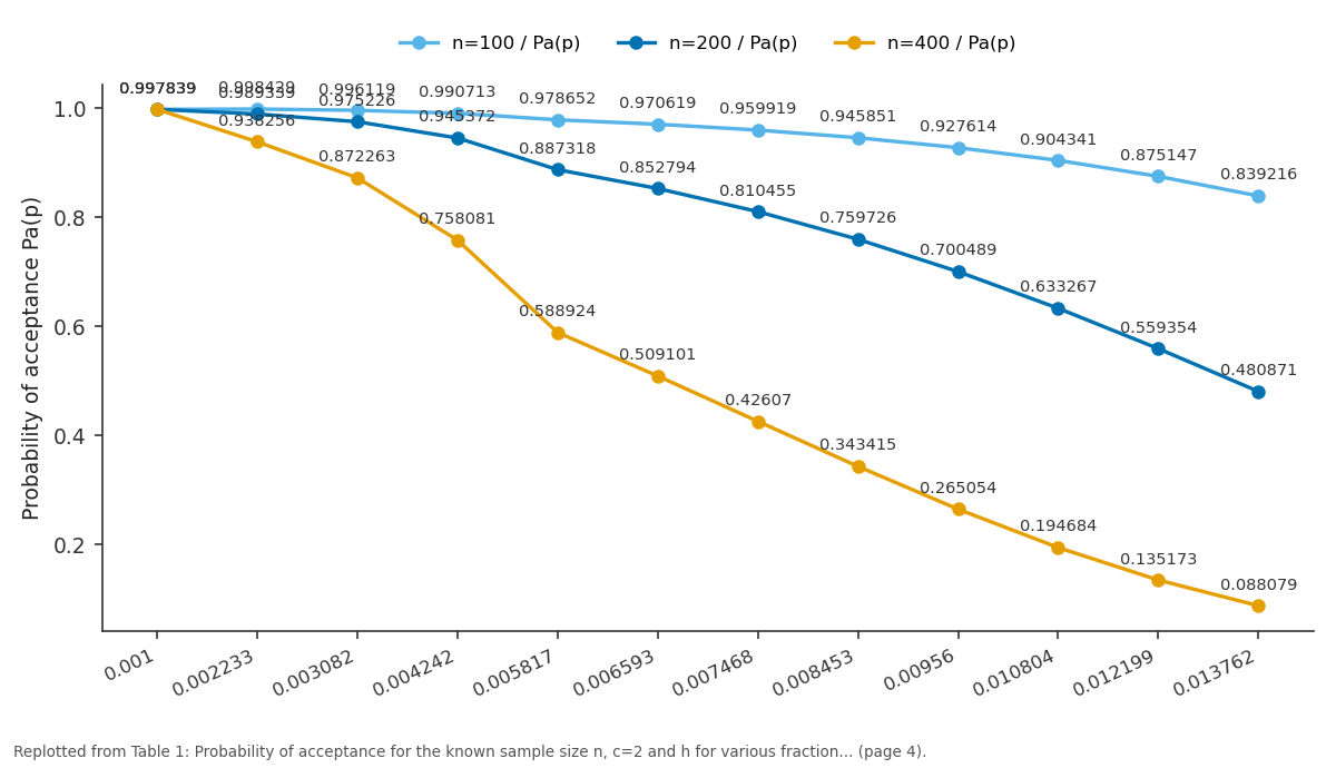
n=100 / Pa(p) and n=200 / Pa(p) and more: 0.001 vs 0.002233 vs 0.003082 vs 0.004242 vs 0.005817
Replotted from Table 1 (page 4) of the original paper. Every bar is the paper's own table value.
View source evidence ↗Figures & tables
From the original paper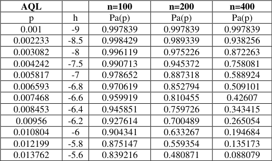 Table 1
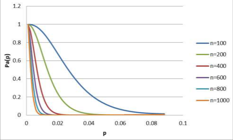 Figure 1
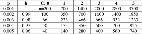 Table 2
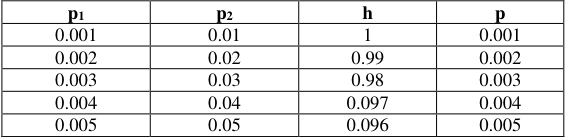 Table 2A
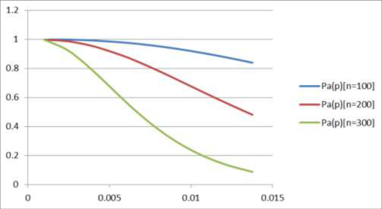 Figure 2
Introduction
In single sampling plan the decision about accepting or rejecting lot is taken on basis of single sample result only and hence it is the most economical plan. But at the same time based on single sample, sometimes rejection of lots may be high even for a small deviation in the quality. Hence single sampling plans faces some shortcomings and may affect the goodwill of the producer. In the case of sequential sampling plan, sample items are examined one at time and after each time inspected one of three decisions is made. viz., to accept the lot, to reject lot or to continued sampling. But inspection of one or two items cannot lead to a good decision until sequences of m units are tested. In fact sequential process ultimately terminates with probability one. Thus sequential sampling plan also faces few drawbacks. Therefore to offset these shortcomings blending of Single and Sequential sampling (SSS) inspection is employed in the quality control inspection. This gives more protection to the Producer and at the same time if the first stage fails consumer is also satisfied with the procedure of unit by unit inspection in the second stage. Therefore the blend of single and sequential sampling plans is more advantages for producer and consumer as well. Prof. Dodge (1969) have classified acceptance sampling into four broad categories. They are lot-by-lot sampling by attributes, lot-by-lot sampling by variables, Continuous Sampling by attributes or variables and Special purpose sampling plans. Hamaker (1960), insist during designing a sampling plan one has to exert pressure on the producer when the quality of the lot is unreliable. Peach and Littauer (1946) have given tables to determine the parameters of the single sampling plan for the known producer and consumer risks. Guenther (1978) [8] has developed a search procedure for finding the parameters of sampling plans. Golub (1953) [6] has given a method for finding the sampling plans by minimizing the sum of the risks. Cameron (1952) [1] , has constructed tables for selection of single sampling plans. Dodge and Romig (1959) have constructed tables for single sampling plans indexed through LTPD. Schilling (1967) [2] has contributed to new type of designing procedure. Hald (1981) [9] , has given construction of sampling plans for attribute quality characteristics. Wald (1947) [14] , has developed sequential sampling protocol and determined the parameters. Suresh and Devaarul (2012), have developed mixed sampling plans for chain of lots. Devaarul and Edna (2011) [3] , have developed sampling plans for costly products. Devaarul
SSS-algorithm for sentencing the lots. First stage
Step 1: Draw a random sample of size n from the lot. Let it be first stage.
Step 2: Count the number of defectives d.
Step 3: If d ≤ c, then accept the lot.
Step 4: If d >c, do not reject the lot, but go to the second stage of inspection.
Second stage
Step 5: Now sequential sampling inspection is implemented in the second stage.
Step 6: Select and examine one item at a time. At m th stage of inspection determine.
Where p 1 , p 2 be the probabilities of getting d m defectives in the sample of size m under AQL and LQL respectively. Let A=(1-ß)/α and B=ß/(1-α)
Step 7: If 𝜆 𝑚 ≤ B, accept the lot.
Step 8: If 𝜆 𝑚 ≥ A, reject the lot.
Step 9: B < 𝜆 𝑚 < A, continue the item by item inspection and follow step5 onwards.
Step 10: For computational points of view, it would be much easier to deal with log 𝜆 𝑚 rather than with 𝜆 𝑚 .
Thus, sequential sampling can be restated as follows i) If log𝜆 𝑚 ≥ log A, reject the lot ii) If log 𝜆 𝑚 ≤ log B, accept the lot, and iii) If log B < log 𝜆 𝑚 < log A, continue sampling by taking one more observation iv) log 𝜆 𝑚 =d m log (
Proof:
The lot may be accepted in following cases Case (i) Take a sample of size "n" from the lot i) If d=0, accept the lot ii) If d=1, accept the lot If d=c, accept the lot Otherwise case (ii) is followed.
Case (ii)
Case (ii)
Average sample number
The average sample number (ASN) is the expected value of sample size required for making a decision about the acceptance or rejection of the lot.
Theorem
The ASN of new sampling plan is as follows:
Proof:
We know that ASN=E(n) Two cases, case(i) and case(ii) Step 1: The designing procedure of (SSS) indexed through AQL and LTPD are given P a (𝑝 1 ) ≥ β 1 and P a (𝑝
Step 2: Using Schilling's (1967) [2] designing procedure, split the probability of acceptance for the first and second stages. Let it be β 1 ' and β 1 " at AQL and β 2 ' and β 2 " at LQL.
Step 3: Determine the first stage inspection parameters for the known probability of acceptance.
Step 4: Determine the second stage inspection parameter based on second stage probability of acceptance.
Step 5: If p 1 and p 2 are known, then by using the sequential sampling protocol one can determine the process average p.
Using the above designing procedure, tables are constructed for easy implementation in industries.
Interpretation of figures
From the figure (1) and (2), it is found that Probability of acceptance has good shoulder effect when the sample size is lesser. It is advantageous for the producer. Similarly when the inspection of items is more, then OC curve is steep which indicates the sampling plan discriminate between good and bad lots. This may be appreciated and welcome by the consumer.
Illustration
A company's quality control section has to select a SSS sampling plans. The process average is 0.2% and the allowable defective in the first stage of inspection is one. Determine the parameters of SSS plans.
Solution:
Since the AQL = p = 0.2%, from table (2), the SSS plans parameters are n = 350 c=1 h =0.99
Operating procedure of SSS plans First stage
Step 1: Draw a random sample of size n=350 from the lot. Let it be first stage.
Step 2: Count the number of defectives d.
Step 3: If d ≤ 1, then accept the lot.
Step 4: If d >1, do not reject the lot, but go to the second stage of inspection.
Second stage
Step 5: Now sequential sampling inspection is implemented in the second stage.
Step 6: Select and examine one item at a time. At m th stage of inspection, determine Step 7: Since, 0.05 < 𝜆 𝑚 < 9.5, continue the item by item inspection and follow step5 onwards until the lot is either accepted or rejected.
Conclusion
In this paper, a new sampling algorithm by blending single and sequential sampling techniques is developed. The proposed novel algorithm sentence the lot very effectively with an ease of producer risk. This plan also reduces the burden of consumer since item by item inspection is followed if the first stage inspection fails to accept the lot. Based on the novel algorithm, the efficiency measures such as operating characteristics function, Average Sample Number, Average Total Inspection and its Average Outgoing Quality are derived. When the quality deteriorates the probability of acceptance of the lot is lesser compared to ordinary Single Sampling Plans. This gives more pressure on the producer to maintain the quality. But at the same circumstances, if the lot is not accepted based on the first stage sample, then another chance is given for the producer through item by item inspection. Hence this SSS sampling plan is advantage for both producer and a well as consumer. Since the sampling protocol is simple, it is can be implemented in modern industries.
Figures and tables from the paper
| AQL | — | n=100 | n=200 | n=400 |
|---|---|---|---|---|
| p | h | Pa(p) | Pa(p) | Pa(p) |
| 0.001 | -9 | 0.997839 | 0.997839 | 0.997839 |
| 0.002233 | -8.5 | 0.998429 | 0.989339 | 0.938256 |
| 0.003082 | -8 | 0.996119 | 0.975226 | 0.872263 |
| 0.004242 | -7.5 | 0.990713 | 0.945372 | 0.758081 |
| 0.005817 | -7 | 0.978652 | 0.887318 | 0.588924 |
| 0.006593 | -6.8 | 0.970619 | 0.852794 | 0.509101 |
| 0.007468 | -6.6 | 0.959919 | 0.810455 | 0.42607 |
| 0.008453 | -6.4 | 0.945851 | 0.759726 | 0.343415 |
| 0.00956 | -6.2 | 0.927614 | 0.700489 | 0.265054 |
| 0.010804 | -6 | 0.904341 | 0.633267 | 0.194684 |
| 0.012199 | -5.8 | 0.875147 | 0.559354 | 0.135173 |
| 0.013762 | -5.6 | 0.839216 | 0.480871 | 0.088079 |
Table text extracted from the original PDF; superscript letters are shown inline. The original table image is below.
View original table image
| p | h | C: 0 | 1 | 2 | 3 | 4 | 5 |
|---|---|---|---|---|---|---|---|
| 0.001 | 1 | n=200 | 700 | 1400 | 2000 | 2800 | 3700 |
| 0.002 | 0.99 | 100 | 350 | 700 | 1000 | 1400 | 1850 |
| 0.003 | 0.98 | 66 | 233 | 466 | 666 | 933 | 1233 |
| 0.004 | 0.97 | 50 | 175 | 350 | 500 | 700 | 925 |
| 0.005 | 0.96 | 40 | 140 | 280 | 400 | 560 | 740 |
Table text extracted from the original PDF; superscript letters are shown inline. The original table image is below.
View original table image
| p1 | p2 | h | p |
|---|---|---|---|
| 0.001 | 0.01 | 1 | 0.001 |
| 0.002 | 0.02 | 0.99 | 0.002 |
| 0.003 | 0.03 | 0.98 | 0.003 |
| 0.004 | 0.04 | 0.097 | 0.004 |
| 0.005 | 0.05 | 0.096 | 0.005 |
Table text extracted from the original PDF; superscript letters are shown inline. The original table image is below.
View original table image
References
14 in the original paper- Cameron. Tables for Constructing and for computing the operating characteristics of single sampling plans, IQC 195237-39 1952.
- Edward G. Schilling, Acceptance Sampling in Quality Control, Centre for Quality and Applied Statistics Rochester Institute Of Technology Rochester, New York 1967.
- Deva Arul S, Rebecca Jebaseeli Edna K. Mixed Sampling Product Control for costly or destructive items, Journal of Mathematical Sciences and Computer Applications 2011;1(3):85-94.
- Devaarul S, Vijila M. Design and Development of Relational Chain Sampling Plans [RChSP(0,i)] for attribute quality characteristics, Cogent Mathematics, USA 4-1408232:1-8 2017.
- Dodge. Statistical Control in Sampling Inspection, American Mechanist, 1932, 1085-88.
- Golub A. Designing single-sampling inspection plans when the sample size is fixed. Journal of American Statistical Association 1953;48:278-288.
- Guenther WC. Use of the Binomial, Hypergeometric and Poisson tables to obtain Sampling Plans, Journal of Quality Technology 1969;1(2):105-109.
- Guenther WC. Sampling Inspection in Statistical Quality Control, McMillan, New York 1978.
- Hald A. Statistical theory of sampling inspection by attributes, Academic Press, New York 1981.
- Ramya and Devaarul. Design and Development of Reliability Sampling Plans for Intermittent Testing Based on Type-I Censoring, International Journal of Applied Engineering Research 2017;12(24):15319-15325. ISSN 0973-4562.
- Suresh KK, Devaarul S. Designing and Selection of Mixed Sampling Plans with Chain Sampling as attribute plan, Quality Engineering, Journal of American Society for Quality, U.S.A 2002;15(1):155-160.
- Suresh KK, Devaarul S. Combining Process and Product Control for Reducing Sampling Costs, Economic Quality Control, Journal and Newsletter for Quality and Reliability-Germany 2002;17(2):87-194.
- Suresh KK, Devaarul S. Multi-Dimensional Mixed Sampling Plans, Journal of Quality Engineering, U.S.A 2003;16(2):233237.
- Wald A. Sequential Analysis, John Wiley, New York (Reprinted Dover Publications, New York 1947, 1973.