
Research article · 2020 · Full text
International Journal of Statistics and Applied MathematicsUse of the theory of Euclidean distance in testing for multivariate normality with application to breast cancer diagnostic data
Volume 5(5) · Pages 128–134
Research areasStatistical Distribution Estimation and ApplicationsStatistical Methods and Bayesian InferenceBayesian Methods and Mixture Models
Abstract
Author-writtenThis paper presents an adaptive technique for assessing multivariate normality (MVN). It is shown that the squared L2¬ norm otherwise known as the squared Euclidean distance of a standard d-variate normal distribution is chi-squared distributed with d degrees of freedom. Based on this, an adaptive test for MVN was proposed as the sum of squared differences between the ordered set of the squared normalized L2 norms of the observation vectors and the set of the population pth quantiles from the chi-squared distribution with d degrees of freedom. The critical values of the test were evaluated for different sample sizes and different number of random variables contained in the multivariate data through extensive simulations. For some selected sample sizes and number of random variables, the empirical power of the proposed test was compared with those of some other widely used techniques for assessing multivariate normality. The results showed that the test can be recommended as a good tool for testing MVN of a dataset especially for large sample cases. The test was applied to a data set extracted from the Wisconsin breast cancer diagnostic data and the result showed that the data set was not multivariate normal.
Summary
Source-checkedPlain-language reading of the full paper, prepared with AI and checked against the text. Each point links to the authors' own words.
Why it matters
- Many existing MVN tests rely on different mathematical characterizations, including characteristic functions, moment generating functions, and measures of skewness or kurtosis. View evidence ↗
The question
- The study aims to develop a new test for multivariate normality using a chi-squared transform based on the principle of Euclidean distance. View evidence ↗
What they did
- The proposed test calculates the sum of squared differences between ordered squared normalized L2 norms of observation vectors and the population quantiles of a chi-squared distribution with d degrees of freedom. View evidence ↗
What they found
- The proposed L2n,d test demonstrated strong control over the type-I error rate across all tested sample sizes and dimensions. View evidence ↗
- At small sample sizes, the proposed test was generally not more powerful than the other competing MVN tests. View evidence ↗
- For sample sizes greater than 50, the proposed test's power was at least as good as any other competing technique for nearly all alternative distributions at dimensions d=2 and d=5. View evidence ↗
- The test showed a progressive increase in power as sample size grew, achieving the highest average power among the tests at n = 500 for both dimensions. View evidence ↗
- When applied to a breast cancer diagnostic dataset (n=500, d=5), the test statistic of 15835.78 far exceeded the critical value of 72.8074, indicating the data is not multivariate normal. View evidence ↗
What it means
- The authors recommend the L2n,d test as an effective tool for testing multivariate normality due to its competitive power and strong control over type-I errors. View evidence ↗
Visual summary
3 visualsIllustrations explain the paper; charts are replotted from the paper's own table values.
L2n,d Test Logic
AI-generated conceptual illustration (breast cancer tissue biopsy samples). It explains the idea and does not show study data.
View source evidence ↗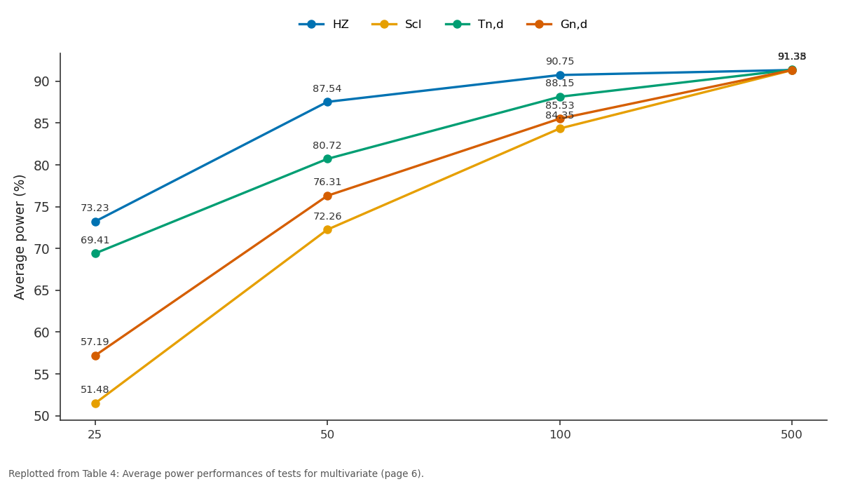
HZ and Scl and more: 25 vs 50 vs 100 vs 500
Replotted from Table 4 (page 6) of the original paper. Every bar is the paper's own table value.
View source evidence ↗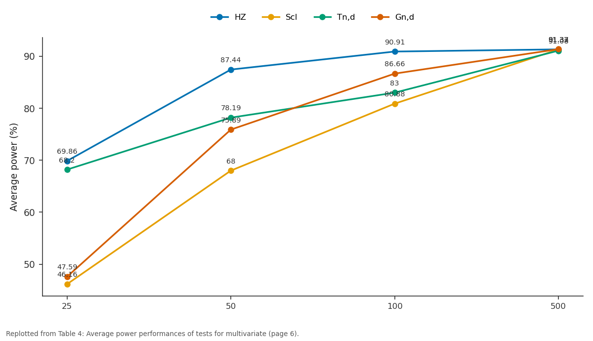
HZ and Scl and more: 25 vs 50 vs 100 vs 500
Replotted from Table 4 (page 6) of the original paper. Every bar is the paper's own table value.
View source evidence ↗Figures & tables
From the original paper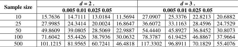 Table 1
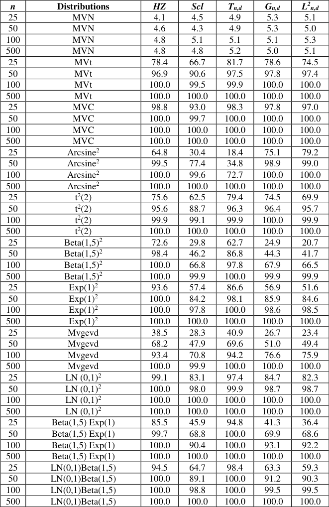 Table 2
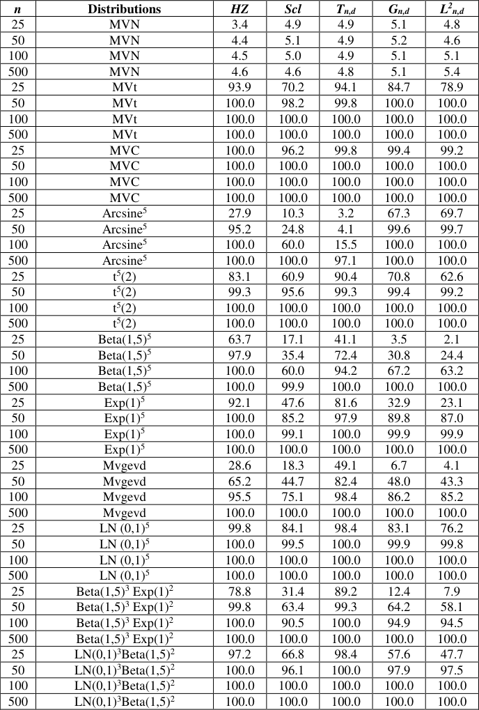 Table 3
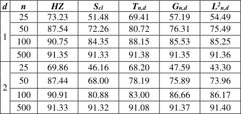 Table 4
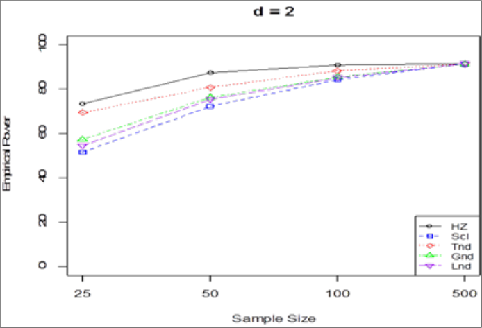 Figure 1
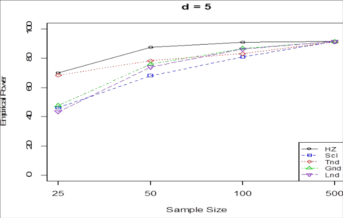 Figure 2
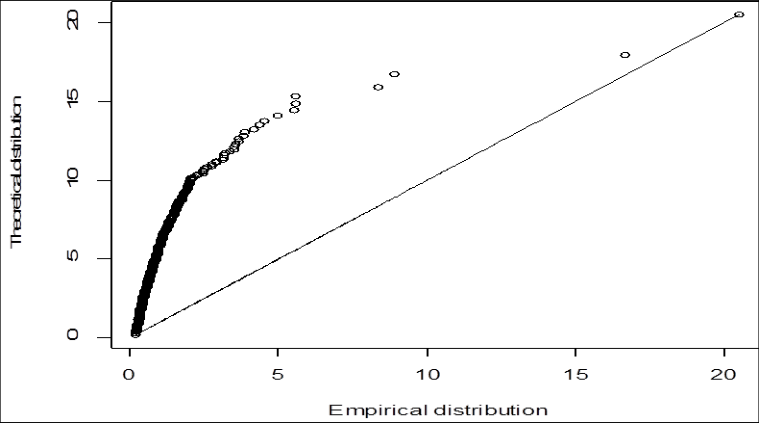 Figure 3
Introduction Suppose a d-component random vector
is defined by a distribution function () F x with probability function () f x . Let 0 () F x be a distribution function of a multivariate normal population having mean vector μ and covariance matrix Σ , with probability density function 0 () f x . Suppose a sample of n independent and identically distributed (iid) observation vectors 1 2 , , ..., n x x
x is available from an unknown continuous distribution function ( ) F x . Testing the assumption of multivariate normality (MVN) of the data set involves a statistical determination of whether or not the unknown distribution function ( ) F x conforms to the known distribution function 0 () F x . There is no shortage of procedures for obtaining goodness-of-fit test for MVN. This is made possible by the various characterizations of the multivariate normal distribution such as the characteristic function, the moment generating function, the Laplace transform as well as measures of entropy, skewness and kurtosis. In fact, several different statistics have been developed for assessing MVN by the use of each of these and many other characterizations. This therefore presents these procedures in classes according to each characterization. Some of the tests include Kuwana and Kariya [1] ; Baxter and Gale [2] ; Dufour, Khalaf and Beaulieu [3] and Koizumi, Hyodo and Pavlenko [4] . One class of tests for MVN of multivariate datasets that have received attention of researchers is the probability plots class of tests for MVN. Suppose 1 2 , , ..., n x x
x is a random sample of n observation vectors from a d-dimensional multivariate normal population having mean vector μ and covariance matrix . Let x and S be estimators of μ and Σ respectively. It is well known that the squared radii 1 ( ) ( ); 1, 2, ..., (1) are asymptotically distributed as a chi-squared distribution with d degrees of freedom, where
Healy [5] obtained a graphical plot of the ordered squared radii, () ; 1, 2, . . ., j y j n versus the approximate expected order statistics from the chi-squared distribution with d degrees of freedom. As a means of assessing MVN of the data set, he stated that the MVN of the data set may be rejected if the plot fails to be approximately linear. Madukaife and Okafor [6] used this transformation to obtain a formal test for MVN based on probability plots. They ordered the squared radii to have the order statistics . Precisely, their test statistic is the sum of squared differences between the observed and corresponding expected order statistics. They concluded that multivariate normality of a data set will be rejected for large values of the statistic. It is important to note that the squared radii given in (1) are obtained by the principle of sample Mahalanobis squared distance of multivariate observations. On the assumption of multivariate normality, the sample Mahalanobis squared distance is not the only transform that gives rise to a set of chi-square observations with d degrees of freedom. This paper proposes to obtain another chisquared transform by the principle of Euclidean distance which can be adapted to the test statistic according to Madukaife and Okafor [6] . The rest of the paper is organized as follows: the technique is proposed in the immediate next section while the empirical critical values of the proposed test follow after it as a section. Thereafter, the powers of the test are compared with the powers of other good omnibus tests for MVN in the literature. The proposed test is applied to a real-life data set and finally, the paper ends with the concluding section
The proposed test
μΣ . The L2 norm of x , also known as the Euclidean distance or Euclidean norm of the vector, is defined by
x . The squared Euclidean distance
x is simply sum of squares of dependent normal random variables. Kettani and Ostrouchov [7] have obtained the distribution of this xx for different forms of μ and Σ . Precisely, they obtained the characteristic function of this univariate transform as:
The characteristic function in (2) reduces to
which is that of chi-squared distribution with d degrees of freedom when and let μ 0 and Σ be estimated by x and S respectively, then
is the jth observation of the ith principal component of x , where i h is the normalized eigenvector associated with the ith estimated eigenvalue of the random vector x . Hanusz and Tarasinska [8] standardized the ij y observations in each ith principal component given in (3) in order to have observations that do not depend on the sample covariance matrix S and obtained () ; 1, 2, . . ., ; 1, 2, . . ., ( 1)
such that under the assumption of multinormality of x, ij z will be a jth observation of ith approximately independent standard normal principal component of x. Now, let a random sample of n observation vectors be transformed to ; 1, 2, . . ., ;
is the jth chi-squared observation with d degrees of freedom. The ' j w s are ordered as (1) (2) ( ) ...
with their corresponding approximate expected chi-squared order statistics ; 1, 2, . . ., A test for MVN, adapted from Madukaife and Okafor [6] is therefore proposed as the sum of squared differences between each observed chi-squared value and the corresponding approximate expected chi-squared value. That is, the proposed statistic is
The test rejects multivariate normality of the data set for large value of the statistic.
Empirical critical values of the test
The empirical critical values of the test statistic for different combinations of the sample size n and the number of variables d through extensive simulation studies are obtained here. Precisely, the critical values at 0.5, 1, 2. 1. ) is compared with the powers of some other omnibus tests for MVN most of which are based on the probability plots and the comparison is made through extensive simulation studies. The competing tests considered here include the Henze and Zirkler (HZ) test for MVN, Henze and Zirkler [9] ; the Singh's classical (Scl) test for MVN, Singh [10] ; the Madukaife and Okafor ( , nd T , , n d G ) tests for multivariate normality, Madukaife and Okafor [11,6] . The competing test procedures are described in what follows.
Description of the competing test statistics
Henze and Zirkler Test: Henze and Zirkler [9] obtained a class of affine invariant and consistent test for multivariate normality based on the distance between the empirical characteristic function and the theoretical characteristic function of the multivariate normal distribution. The statistic is of the form , , (4 ( is singular) ( is nonsingular))
; I(.) is an indicator function and S is the sample covariance matrix of the multivariate data set. They recommended the smoothing parameter, to be obtained from kernel density estimation by Singh's Classical Test: Singh [10] obtained a classical test for multivariate normality based on the product moment correlation coefficient between an ordered beta transform, () ; 1, 2, . . .,
of a multivariate data set and the set of expected beta order statistics, ; 1, 2, . . .,
. The beta of the first kind transform was obtained according to Gnanadesikan and Kettenring [12] by further transforming ;
. They concluded that multivariate normality of the data set will be rejected if the correlation coefficient is not close to 1. The correlation coefficient test statistic is given as:
; . Also, the critical values for this test were obtained empirically via simulation studies.
Madukaife and Okafor Tn,d and Gn.d Tests: Madukaife and
Okafor [11,6] respectively obtained two tests for assessing the assumption of MVN of multivariate data sets. The test procedures have the statistics: 2 () 11 ( )
, where () ij z is the jth sample order statistic in the ith principal component obtained from the multivariate data set according to (4), ( ) j y is the jth sample order statistic of the chi squared transform observations according to (1). In each statistic, j c is the jth expected order statistic. They obtained the critical values of the tests empirically via extensive simulation studies said that MVN of data sets are rejected for large values of the statistics.
Power Comparison of the Tests
In this section, 10,000 data sets were generated in each combination of n = 25, 50, 100 and 500 and d = 2 and 5 from 11 different multivariate distributions. The values of each of the competing statistics being compared were evaluated in each of the 10,000 simulated samples for each n and d. The empirical power of each test statistic was obtained as the percentage of the 10,000 samples that is rejected by the statistic at of 5%. The distributions include the standard multivariate normal distribution (MVN); the multivariate Cauchy distribution (MVC) with identity covariance matrix; the multivariate t distribution (MVt) with identity covariance matrix and 2 degrees of freedom and multivariate generalized extreme value distribution (Mvgevd) with dependent parameter 0.72. Others are products of some univariate distributions such as student's t with 2 degree of freedom, standard lognormal, beta of the first kind with 1 and 5 parameters, standard exponential, standard arcsine and standard normal. The power performance is presented in Tables 2 and3 respectively for d = 2 and 5. From Tables 2 and3, it is expectedly observed a general rise in power with increase in sample size in all the test statistics and in all the distributions considered except the standard multivariate normal. Under this standard multivariate normal distribution, it is expected that the power will be equal to the nominal of 5%. This amounts to type I error rate since the null distribution of multivariate normality is true. The proposed L 2 n,d test together with the Tn,d and Gn,d tests maintained this in all the sample sizes and variable dimensions considered showing that it has a very good control over type-1 error rate. Also, the proposed test failed to be generally more powerful than the rest of the competing tests especially at small sample sizes. However, at large sample sizes of more than 50, the power performances of the proposed test no doubt were generally at worst as good as any other competing technique in almost all the alternative distributions considered both at d = 2 and d = 5. Again, no much difference in the pattern of power behaviour of the proposed test was recorded at difference variable dimensions. The test therefore can be recommended as a very powerful technique for assessing multivariate normality of data sets especially at large sample sizes. In order to make for a better comparison, the average power performances of these competing tests are obtained for each sample size and number of variables involved. Often times in comparisons of this nature, consideration has always been given to the nature of the alternative distribution, in terms of symmetry, see Thulin [13] for instance. However in practice, the nature of the distribution whose multinormality is in question is usually not known. As a result, the symmetry of the distributions is ignored and the average powers of the competing tests on all the 11 distributions considered are obtained as presented in Table 4. The power plots in terms of the average powers are also presented in Figures1 and 2 respectively for the number of variables 2 and 5.
| d | n | HZ | Scl | Tn,d | Gn,d | L2 n,d |
|---|---|---|---|---|---|---|
| 1 | 25 | 73.23 | 51.48 | 69.41 | 57.19 | 54.49 |
| 50 | 87.54 | 72.26 | 80.72 | 76.31 | 75.49 | |
| 100 | 90.75 | 84.35 | 88.15 | 85.53 | 85.25 | |
| 500 | 91.35 | 91.33 | 91.38 | 91.35 | 91.36 | |
| 2 | 25 | 69.86 | 46.16 | 68.20 | 47.59 | 43.30 |
| 50 | 87.44 | 68.00 | 78.19 | 75.89 | 73.96 | |
| 100 | 90.91 | 80.88 | 83.00 | 86.66 | 86.17 | |
| 500 | 91.33 | 91.32 | 91.08 | 91.37 | 91.40 |
Table text extracted from the original PDF; superscript letters are shown inline. The original table image is below.
View original table image
From Table 4 and Figures 1 and2, the newly proposed test gives a competitive power performance. Its power performance appears to be inferior to other tests at small sample size of 25 except for the Scl test. However, it maintained a progressive power gain along the direction of increasing sample size that at n = 500, its powers came top in averagely both variable dimensions.
Application of the L 2 n,d test to the breast cancer data
In order to show the applicability of the proposed test to realife data sets, a 500 observation vectors with 5-component data set was extracted from a 32-component breast cancer diagnostic data set, retrieved from www.world/datasets/multivariate [14] . Each variable in the data set represents a characteristic of the cell nuclei present in images of a fine needle aspirate (FNA) of a breast mass. In order to test for multivariate normality of the extracted data set, an R statistical code for the L2 statistic gave the value of the statistic as 15835.78 against the critical value of the statistics at = 0.05 with n = 500 and d = 5 which is 72.8074. This shows clearly that the data set is not multivariate normal at = 0.05. The result of the test is supported with the quantile-quantile plot of the chi-squared transformed form of the data, which is expected to be linear if the data set is actually multivariate normal, see Figure 3 below. The proposed statistic is an alternative to the Gn,d statistic according to Madukaife and Okafor [11] . From the power comparisons carried out in this work, the proposed L 2 n,d test, no doubt, can be recommended for use as a good tool for testing multinormality, having a very strong control over type-I error as well as highly competitive power.
Figures and tables from the paper
| Sample size | d = 2 . | — | — | — | d = 3 . | — | — | — |
|---|---|---|---|---|---|---|---|---|
| 0.005 0.01 0.025 0.05 | 0.005 0.01 0.025 0.05 | |||||||
| 10 | 15.7636 | 14.7111 | 13.0184 | 11.5694 | 27.0907 | 25.3376 | 22.8213 | 20.6882 |
| 25 | 27.9985 | 24.3414 | 20.0024 | 16.8647 | 36.6072 | 33.1163 | 28.4596 | 24.7529 |
| 50 | 49.8609 | 39.0805 | 28.5069 | 22.9887 | 54.4440 | 45.8927 | 36.8452 | 30.8073 |
| 100 | 71.6042 | 55.4426 | 38.7936 | 30.0632 | 78.3787 | 61.9425 | 46.8867 | 37.9664 |
| 500 | 101.1215 | 81.9565 | 60.7241 | 46.4818 | 117.3302 | 96.8911 | 70.1829 | 55.4076 |
Table text extracted from the original PDF; superscript letters are shown inline. The original table image is below.
View original table image
| n | Distributions | HZ | Scl | Tn,d | Gn,d | L2 n,d |
|---|---|---|---|---|---|---|
| 25 | MVN | 4.1 | 4.5 | 4.9 | 5.3 | 5.1 |
| 50 | MVN | 4.6 | 4.3 | 4.9 | 5.3 | 5.0 |
| 100 | MVN | 4.8 | 5.1 | 5.1 | 5.1 | 5.3 |
| 500 | MVN | 4.8 | 4.8 | 5.2 | 5.0 | 5.1 |
| 25 | MVt | 78.4 | 66.7 | 81.7 | 78.6 | 74.5 |
| 50 | MVt | 96.9 | 90.6 | 97.5 | 97.8 | 97.4 |
| 100 | MVt | 100.0 | 99.5 | 99.9 | 100.0 | 100.0 |
| 500 | MVt | 100.0 | 100.0 | 100.0 | 100.0 | 100.0 |
| 25 | MVC | 98.8 | 93.0 | 98.3 | 97.8 | 97.0 |
| 50 | MVC | 100.0 | 99.7 | 100.0 | 100.0 | 100.0 |
| 100 | MVC | 100.0 | 100.0 | 100.0 | 100.0 | 100.0 |
| 500 | MVC | 100.0 | 100.0 | 100.0 | 100.0 | 100.0 |
| 25 | Arcsine2 | 64.8 | 30.4 | 18.4 | 75.1 | 79.2 |
| 50 | Arcsine2 | 99.5 | 77.4 | 34.8 | 98.9 | 99.0 |
| 100 | Arcsine2 | 100.0 | 99.6 | 72.7 | 100.0 | 100.0 |
| 500 | Arcsine2 | 100.0 | 100.0 | 100.0 | 100.0 | 100.0 |
| 25 | t2(2) | 75.6 | 62.5 | 79.4 | 74.5 | 69.9 |
| 50 | t2(2) | 95.6 | 88.7 | 96.3 | 96.4 | 95.7 |
| 100 | t2(2) | 99.9 | 99.1 | 99.9 | 100.0 | 99.9 |
| 500 | t2(2) | 100.0 | 100.0 | 100.0 | 100.0 | 100.0 |
| 25 | Beta(1,5)2 | 72.6 | 29.8 | 62.7 | 24.9 | 20.7 |
| 50 | Beta(1,5)2 | 98.4 | 46.2 | 86.8 | 44.3 | 41.7 |
| 100 | Beta(1,5)2 | 100.0 | 66.8 | 97.8 | 67.9 | 66.5 |
| 500 | Beta(1,5)2 | 100.0 | 99.9 | 100.0 | 99.9 | 99.9 |
| 25 | Exp(1)2 | 93.6 | 57.4 | 86.6 | 56.9 | 51.6 |
| 50 | Exp(1)2 | 100.0 | 84.2 | 98.1 | 85.9 | 84.6 |
| 100 | Exp(1)2 | 100.0 | 97.8 | 100.0 | 98.6 | 98.5 |
| 500 | Exp(1)2 | 100.0 | 100.0 | 100.0 | 100.0 | 100.0 |
| 25 | Mvgevd | 38.5 | 28.3 | 40.9 | 26.7 | 23.4 |
| 50 | Mvgevd | 68.2 | 47.9 | 69.6 | 51.0 | 49.4 |
| 100 | Mvgevd | 93.4 | 70.8 | 94.2 | 76.6 | 75.9 |
| 500 | Mvgevd | 100.0 | 99.9 | 100.0 | 100.0 | 100.0 |
| 25 | LN (0,1)2 | 99.1 | 83.1 | 97.4 | 84.7 | 82.3 |
| 50 | LN (0,1)2 | 100.0 | 98.0 | 99.9 | 98.7 | 98.7 |
| 100 | LN (0,1)2 | 100.0 | 100.0 | 100.0 | 100.0 | 100.0 |
| 500 | LN (0,1)2 | 100.0 | 100.0 | 100.0 | 100.0 | 100.0 |
| 25 | Beta(1,5) Exp(1) | 85.5 | 45.9 | 94.8 | 41.3 | 36.4 |
| 50 | Beta(1,5) Exp(1) | 99.7 | 68.8 | 100.0 | 69.9 | 68.6 |
| 100 | Beta(1,5) Exp(1) | 100.0 | 90.4 | 100.0 | 93.1 | 92.2 |
| 500 | Beta(1,5) Exp(1) | 100.0 | 100.0 | 100.0 | 100.0 | 100.0 |
| 25 | LN(0,1)Beta(1,5) | 94.5 | 64.7 | 98.4 | 63.3 | 59.3 |
| 50 | LN(0,1)Beta(1,5) | 100.0 | 89.1 | 100.0 | 91.2 | 90.3 |
| 100 | LN(0,1)Beta(1,5) | 100.0 | 98.8 | 100.0 | 99.5 | 99.5 |
| 500 | LN(0,1)Beta(1,5) | 100.0 | 100.0 | 100.0 | 100.0 | 100.0 |
Table text extracted from the original PDF; superscript letters are shown inline. The original table image is below.
View original table image
| n | Distributions | HZ | Scl | Tn,d | Gn,d | L2 n,d |
|---|---|---|---|---|---|---|
| 25 | MVN | 3.4 | 4.9 | 4.9 | 5.1 | 4.8 |
| 50 | MVN | 4.4 | 5.1 | 4.9 | 5.2 | 4.6 |
| 100 | MVN | 4.5 | 5.0 | 4.9 | 5.1 | 5.1 |
| 500 | MVN | 4.6 | 4.6 | 4.8 | 5.1 | 5.4 |
| 25 | MVt | 93.9 | 70.2 | 94.1 | 84.7 | 78.9 |
| 50 | MVt | 100.0 | 98.2 | 99.8 | 100.0 | 100.0 |
| 100 | MVt | 100.0 | 100.0 | 100.0 | 100.0 | 100.0 |
| 500 | MVt | 100.0 | 100.0 | 100.0 | 100.0 | 100.0 |
| 25 | MVC | 100.0 | 96.2 | 99.8 | 99.4 | 99.2 |
| 50 | MVC | 100.0 | 100.0 | 100.0 | 100.0 | 100.0 |
| 100 | MVC | 100.0 | 100.0 | 100.0 | 100.0 | 100.0 |
| 500 | MVC | 100.0 | 100.0 | 100.0 | 100.0 | 100.0 |
| 25 | Arcsine5 | 27.9 | 10.3 | 3.2 | 67.3 | 69.7 |
| 50 | Arcsine5 | 95.2 | 24.8 | 4.1 | 99.6 | 99.7 |
| 100 | Arcsine5 | 100.0 | 60.0 | 15.5 | 100.0 | 100.0 |
| 500 | Arcsine5 | 100.0 | 100.0 | 97.1 | 100.0 | 100.0 |
| 25 | t5(2) | 83.1 | 60.9 | 90.4 | 70.8 | 62.6 |
| 50 | t5(2) | 99.3 | 95.6 | 99.3 | 99.4 | 99.2 |
| 100 | t5(2) | 100.0 | 100.0 | 100.0 | 100.0 | 100.0 |
| 500 | t5(2) | 100.0 | 100.0 | 100.0 | 100.0 | 100.0 |
| 25 | Beta(1,5)5 | 63.7 | 17.1 | 41.1 | 3.5 | 2.1 |
| 50 | Beta(1,5)5 | 97.9 | 35.4 | 72.4 | 30.8 | 24.4 |
| 100 | Beta(1,5)5 | 100.0 | 60.0 | 94.2 | 67.2 | 63.2 |
| 500 | Beta(1,5)5 | 100.0 | 99.9 | 100.0 | 100.0 | 100.0 |
| 25 | Exp(1)5 | 92.1 | 47.6 | 81.6 | 32.9 | 23.1 |
| 50 | Exp(1)5 | 100.0 | 85.2 | 97.9 | 89.8 | 87.0 |
| 100 | Exp(1)5 | 100.0 | 99.1 | 100.0 | 99.9 | 99.9 |
| 500 | Exp(1)5 | 100.0 | 100.0 | 100.0 | 100.0 | 100.0 |
| 25 | Mvgevd | 28.6 | 18.3 | 49.1 | 6.7 | 4.1 |
| 50 | Mvgevd | 65.2 | 44.7 | 82.4 | 48.0 | 43.3 |
| 100 | Mvgevd | 95.5 | 75.1 | 98.4 | 86.2 | 85.2 |
| 500 | Mvgevd | 100.0 | 100.0 | 100.0 | 100.0 | 100.0 |
| 25 | LN (0,1)5 | 99.8 | 84.1 | 98.4 | 83.1 | 76.2 |
| 50 | LN (0,1)5 | 100.0 | 99.5 | 100.0 | 99.9 | 99.8 |
| 100 | LN (0,1)5 | 100.0 | 100.0 | 100.0 | 100.0 | 100.0 |
| 500 | LN (0,1)5 | 100.0 | 100.0 | 100.0 | 100.0 | 100.0 |
| 25 | Beta(1,5)3 Exp(1)2 | 78.8 | 31.4 | 89.2 | 12.4 | 7.9 |
| 50 | Beta(1,5)3 Exp(1)2 | 99.8 | 63.4 | 99.3 | 64.2 | 58.1 |
| 100 | Beta(1,5)3 Exp(1)2 | 100.0 | 90.5 | 100.0 | 94.9 | 94.5 |
| 500 | Beta(1,5)3 Exp(1)2 | 100.0 | 100.0 | 100.0 | 100.0 | 100.0 |
| 25 | LN(0,1)3Beta(1,5)2 | 97.2 | 66.8 | 98.4 | 57.6 | 47.7 |
| 50 | LN(0,1)3Beta(1,5)2 | 100.0 | 96.1 | 100.0 | 97.9 | 97.5 |
| 100 | LN(0,1)3Beta(1,5)2 | 100.0 | 100.0 | 100.0 | 100.0 | 100.0 |
| 500 | LN(0,1)3Beta(1,5)2 | 100.0 | 100.0 | 100.0 | 100.0 | 100.0 |
Table text extracted from the original PDF; superscript letters are shown inline. The original table image is below.
View original table image
References
13 in the original paper- Kuwana Y, Kariya T. LBI tests for multivariate normality in exponential power distributions. Journal of multivariate analysis 1991;39:117-134.
- Baxter MJ, Gale NH. Testing for multivariate normality via univariate tests: A case study using lead isotope ratio data. Journal of Applied Statistics. 1998;25(5):671-683.
- Dufour J-M, Khalaf L, Beaulieu M-C. Exact skewness - kurtosis tests for multivariate normality and goodness-offit in multivariate regressions with application to asset pricing models. Oxford Bulletin of Economics and Statistics 2003;65:891-906.
- Koizumi K, Hyodo M, Pavlenko T. Modified Jarque - Bera type tests for multivariate normality in a high dimensional framework. Journal of Statistical Theory and Practice 2014;8(2):382-399.
- Healy MJR. Multivariate normal plotting. Applied Statistics 1968;17:157-161.
- Madukaife MS, Okafor FC. A new large sample goodness of fit test for multivariate normality based on chi squared probability plots. Communications in Statistics - Simulation and Computation 2019;48(6):1651-1664.
- Kettani H, Ostrouchov G. On the distribution of the distance between two multivariate normally distributed points. Proceeding of the 7 th Annual Hawaii International Conference on Statistics, Mathematics and Related fields, Honolulu 2005.
- Hanusz Z, Tarasinska J. New tests for multivariate normality based on Small's and Srivastava's graphical methods. Journal of Statistical Computation and Simulation 2012;80(5):513-526.
- Henze N, Zirkler B. A class of invariant consistent tests for multivariate normality. Communications in Statistics -Theory and Methods 1990;19:3595-3618.
- Singh A. Omnibus robust procedures for assessment of multivariate normality and detection of multivariate outliers. In: GP Patil, CR Rao (Eds) Multivariate Environmental Statistics. North Holland, Amsterdam 1993.
- Madukaife MS, Okafor FC. A powerful affine invariant test for multivariate normality based on interpoint distances of principal components. Communications in Statistics-Simulation and Computation 2018;47(5):12641275.
- Gnanadesikan R, Kettenring JR. Robust estimates, residuals, and outlier detection with multiresponse data. Biometrics 1972;28:81-124.
- Thulin M. Tests for multivariate normality based on canonical correlations. Statistical Methods and Applications 2014;23(2):189-208.