Derivation of continuous equations for density of burglars

The discrete model for movement of burglars is given by the equation as: where R(x, t) is assumed to be strictly positive across the whole spatial domain for all t.We can express the relation in terms of discrete spatial laplacian . For this, in continuous limit, we re-express p(x, t) in terms of p(x, t) and R(x, t) R(X, t), p(x, t) p(X, t), where X=lx, l, is a grid spacing

Illustrations explain the paper; they do not show study data.

AI-generated illustration

↗ Enlarge

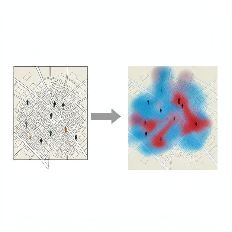
Transition from Discrete to Continuous ModelClose ×

AI-generated conceptual illustration (a city map with stylized human figures representing burglars). It explains the idea and does not show study data.

Open full-size image ↗

Introduction

The discrete model for movement of burglars is given by the equation as:            , ( , ) 1, 2, , R x t x t h x t R x t R x t        R x t ,          x t P x t G h R x t R x t 1, 1 , 2, ,              where ( , ) R x t is assumed to be strictly positive across the whole spatial domain for all t .We can express the relation in terms of discrete spatial laplacian . For this, in continuous limit, we re-express ( , ) x t  in terms of ( , ) X t  and ( , ) ( , ) R x t R X t  , ( , ) ( , ) P x t P X t  , where X lx  , l is a grid spacing. Since probability is independent of length or time scales, therefore we can write ( , ) ( , ) P a X t a P X t  . With this notion and assuming l is small, terms of the above relation can be re-written as 1 ( , ) ( , ) ( , ) ( , ) X x t h t h X t h X t h l l            1 ( , ) ( , ) ( , ) ( , ) X R x t R t R X t R X t l l    Maths 2018; 3(2): 408-411 Md.

Najmul Hoda Research Scholar, Department of Mathematics, T.M. Bhagalpur University, Bhagalpur, Bihar, India Correspondence Md. Najmul Hoda Research Scholar, Department of Mathematics, T.M. Bhagalpur University, Bhagalpur, Bihar, 1 ( 2, ) ( 2, ) ( 2 , ) ( 2 , ) X R x t R t R X l t R X l t l l        R X      X 2     X l R X l R X     1 ( 2, ) ( 2, ) ( 2 , ) ( 2 , ) X R x t R t R X l t R X l t l l        2 2 R X R X l     X    2 2 X l R X l R X       1 ( 1, ) ( 1, ) ( , ) ( , ) X x t t X l t X l t l l                    X 2 1 1 0                 X X 2 R X R X f X X X R X 2 2 4     1 ( 1, ) ( 1, ) ( , ) ( , ) X x t t X l t X l t l l           2     X  R X R X X     2 0 4 ( ) R X   Since ( , ) ( , ) P x t R x t h  therefore,  P x t R x t h ( , ) ( , )       X X 2 R X f l X l R X l R X                 ( , ) ( , ) 2 2 R X R X l X X P t R t h l l     X         X 2 X l R X l R X 2             1 1 ( , ) ( , ) P X t R X t h l l X 2 2 R X l R X X l        X 2 R X l R X 2 ( , ) ( , ) P X t R X t h   ,                 2 th u s 1 , 1 , P x t P X t     2 2 2                      X X        R X l R X R X l X l   4 R X l R X   2       1 , R X t h   2 4 2 2               X     R X l R X l R X X l   4 2 R X l R X         Thus the above relation is reduced to                     R X X l     X X R X t X t h X l t R X l t R X t , , , 2 , ,     R X l R X   2        2 2       X R X t ,        R X R X l X l   X 2        R X l R X   2 X l t R X t h R X l t R X t , 1 , 2 , ,                   G h X 2 2 R X l R X X l        X 2 R X l R X 2                2 2 2 2         X X       R X l R X R X l X l   4  For diffusion of the Risk of victimization and density of burglars to spatial location The relation can be written as R X l R X   2       2   4 2 2       ( , )           X            R X l R X l R X X l   4 R X X t h X l R X l R X 2        R X l R X 2       R X              X l R X h R X l R X 1 2                   X X       R X f l X l R X l R X 2     G h 4 2 R X R X l     X     X 2      X l R X l R X 2       2 R X l R X R X R X l 2 4 2             X X    4        , 1 X t h f l R X h G h       (1)         X l R X l R X 2       2  8 2 2 R X R X l R X l R X           X ( ) w h ere ( ) ( ) ( 2 ) ( ) R X f l X l R X l R X        4        X l R X l R X 2       R X ( )  R X    X l R X l R X ( ) ( 2 ) ( )   X X     X l R X l R X 2         2 2 R X R X l     X    X 2      X l R X l R X 2       Here, (0 ) ( ) f X   2 2 R X R X l     X    X 2       X l R X l R X 2            X R X f l X l R X l R X      2     2 R X l R X R X R X l 2 4 2           X X        2 2 R X R X l 4     X R X 2 X l l R X             2 X l R X l R X 2 2       8 2 2 R X R X l R X l R X           X    4 X l R X l R X 2                       X    l X t h X t X t        X X      2 1 0 2 , , , 2       2 X X X R X R X f X X R X           2 , , R X t X t      X                2 3 2 R X t h G h R X t (1 , ,   X               X X X R X R X R X R X                  X t h X t X t R X t h , , , , 4 1 6 1 6              1 6 X R X     2 R X t X t l     X   X t   X X     2 , , , 2 , R X t   X                     2 2 1     X R X t X t l     X R X t h X t           X X     X X X 2 2 , , , , 2 , R X t   X                     2 4 R X R X X X R X     G h 2 R X R X     X     X  Dividing both sides by h and Taking limit as 0 h  , as 0 l  , 2 2 4 X R X     l 2l  D h 0 2 , and assuming  (constant), we then have 2 2 2               X X X R X R X R X R X R X   X t h X t          4 1 6 1 6    , , lim h  0 1 6 X R X h     2    X X h  0 lim ( , ) ( , ) ( , ) 2 l X t R X t X t h     X X            0            X X X X R X R X f X X X R X R X     2 ( , ) ( , ) R X t X t  X 2         2 2 R X t ( , )     X X X X             2 R X R X X X R X R X     2 R X t X t l     X                      X X 2 , , , , 2 , R X t X t G R X t   X   X     2 0         X X X         R X f X X R X     X t X t R X t , lim , ,       2      t h 0 2 2     X X X     2     2 R X t X t l     X R X R X X X R X R X         X X 2 , , , 2 , X t h R X t   X                  For simplicity, it can be written as 2 R X t X t l     X                      X X X X X X X X X R R R f 2 2 2 2 (0) 2 2 , , , , 2 , R X t X t G R X t   X R R R                         X t X t R X t X t          t X X 2 (0 ) [ ] X X X X R f 1 , , , D , 2 R       2 , , R X t X t      X By maclaurians’ series expansion, we have G R X t ,   X 2 l f l f lf f O l                             As we assumed that density of burglars diffuse to spatial 3 0 0 0 2 ! where 3 ( ) O l represents the terms containing higher power of l .

As l is small, neglecting the term 3 ( ) O l and substituting location, so that ( , ) ( ) X t X    , ( , ) ( ) R X t R X  , thus the equation reduces to     X    R X X X t X     t X X 2 1 , D 2 R X   X the value of (0 ) f , (0 ) f  and (0 ) f  in the above relation, we have                          X  X R X G     R X t X t l f l X t X t      X X 2 2 , , , , 2 , R X t   X   For simplicity the resulting equation can be written as                        (2) With the help of relation (2), the equation (1) can be re- written as R X X X R G t R 1 2 D 2 X                        1 X X X D 2 R D R G t R X                  (3) Note that    2 R R R R R R               ( ) X X          R R R X R X    X X X X X 2   R R R R R R         2    X X X X X 2 R R R R R R          R X R X         Also 2 n 2        X X         d iv X  2 1 i i where  is the discrete spatial laplacian. Using these notations, we can express the above equation (3) as   2 1 D 2 D R R G t R                  (4)

Conclusion

Thus the continuous equation of Risk of victimization field is given by the equation and the continuous equation of density of burglars is given by the equation (4).

1. Brantingham PL, Brantingham PJ. Crime pattern theory. In wortley R, Mazerolle L. editors, Environmental criminology and Crime Analysis. Routledge, 2008.
2. Caldwell RG, Black JA. Juvenile Delinquency The Ronald Press Company, New York, 1971.
3. Calvo-Armengol A, Zenou Y. Social Networks and Crime Decisions: The Role of Social Structure in Facilitating Delinquent Behavior, 2003.
4. Cambel M, Ormerod P. Social interaction and the dynamic of crime, 1998.
5. Felson M, Reachel B. Crime and Everyday Life, 2010.