A comparative study of numerical solutions of second order ordinary differential equations with boundary value problems by shooting method & finite difference method

This study aims at comparing the different time level schemes of different Method to obtain numerical solutions of second order ordinary differential equations. The numerical solutions are obtained for ordinary differential equation with boundary conditions for different values of x. Then the numerical solutions are compared with analytical solution for the considered problem. The comparison of numerical results with the analytical solution reveals that the Finite Difference Method gives the best numerical approximation to analytical solution. The error analysis of different method also discussed. This study can be used to suggest the better accuracy for solving second order ordinary differential equation. This comparative study provides better result for numerical solution of second order ordinary differential equation.

Illustrations explain the paper; charts are replotted from the paper's own table values.

AI-generated illustration

↗ Enlarge

Comparison of Numerical ApproachesClose ×

AI-generated conceptual illustration (mathematical function curves and a coordinate grid). It explains the idea and does not show study data.

Open full-size image ↗

Replotted from source data

↗ Enlarge

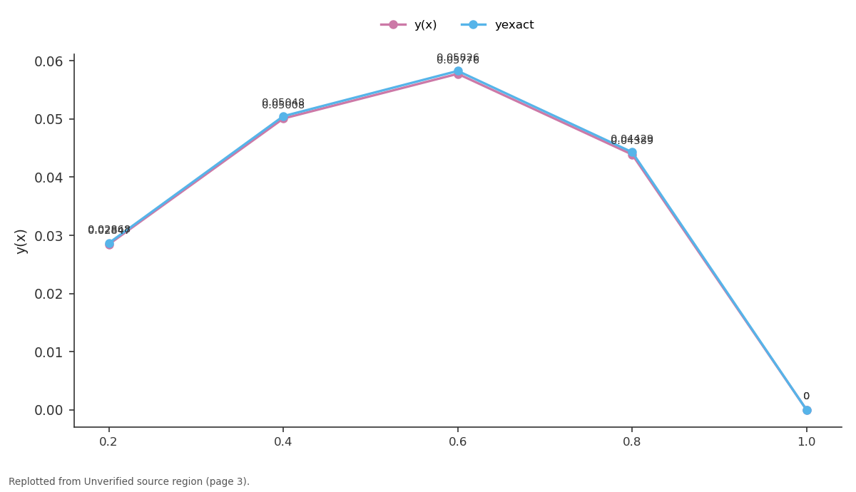
y(x) and yexact: 0.2 vs 0.4 vs 0.6 vs 0.8 vs 1.0Close ×

Replotted from a table (page 3) of the original paper. Every bar is the paper's own table value.

Open full-size image ↗

Results

with the analytical solution reveals that the Finite Difference Method gives the best numerical approximation to analytical solution. The error analysis of different method also discussed. This study can be used to suggest the better accuracy for solving second order ordinary differential equation. This comparative study provides better result for numerical solution of second order ordinary differential equation.

Keywords: Second order differential equation, numerical accuracy, shooting method, finite difference method

Introduction

It is well known that differential equations are in general the backbone of physical system. The physical systems are modeled usually either by ordinary differential or partial differential equation. Various exact and numerical method are available to solve different ordinary and partial differential equations. But in actual practice the variables and coefficients in the differential equation are not crisp.

As those, are obtained by some experiment or experience. So, we need to solve ordinary and partial differential equations accordingly, that is interval ordinary and partial differential equations are to be solved [6]. There are many problems in the field of science, engineering and technology which can be solved by ordinary differential equations formulation. This research will compare the accuracy of various method Shooting Method and Finite Difference Method, in completing numerical solutions of second order ordinary differential equations, which is limited to certain boundary condition [2, 5].

Shooting Method for Boundary Value Problem This method works in three stages i) The given BVP is transferred in two IVPs, ii) Solution of these two IVPs can be determined by Taylor’s series or Runge-Kutta or any other method, iii) Combination of these two solutions is the required solution of the given BVP. Reduction to two IVPs [1]. Let the BVP be ) ( ) ( ' ) ( '' x r y x q y x p y    with   ) (a y and   ) (b y (1) Suppose that ) (x u is the unique solution to the IVP Maths 2019; 4(1): 18-22 Najmuddin Ahmad Department of Mathematics, Integral University, Lucknow, Uttar Pradesh, India Shiv Charan Department of Mathematics, Integral University, Lucknow, Uttar Pradesh, India Correspondence Najmuddin Ahmad Department of Mathematics, Integral University, Lucknow, Uttar Pradesh, India ) ( ) ( ) ( ) (' ) ( '' x r x u x q x u x p u    with   ) (a u and 0 ) ('  a u (2) Furthermore, suppose that ) (x u is the unique solution to the IVP 0 ) ( ) ( ) (' ) ( ''    x v x q x v x p v with 0 ) (  a v and 1 ) ('  a v (3) Then the linear combination ) ( ) ( ) ( 2 1 x v c x u c x y   (4) is the solution of equation 1.1 for some constant 2 1 c , c As   ) (a y and   ) (b y , ) ( ) ( 2 1 a v c a u c    and ) ( ) ( 2 1 b v c b u c    b u c   From the first equation, 1 1  c and From second equation, ) ( ) ( 2 b v Hence equation 1.4 reduces to b u x u x y     [7, 9] (5) ) ( ) ( ) ( x v b v ) ( ) ( This is the solution of the BVP 1.1 and its also satisfies the boundary conditions   ) (a y and   ) (b y Problem 1: x y y   '' with y(0) = 0, y(1) = 0. The second order Runge-Kutta method is used to solve the initial value problem with h = 0.25 Here p(x) = 0, q(x) = 1, r(x) = -x, a = 0, b = 1,  = 0,  = 0.

Now two IVPs are w u  ' with u(0) = 0 x u w   ' and with w(0) = ) 0 ('u = 0 (6) And z v  ' with v(0) = 0 v z  ' and with z(0) = ) 0 ('v = 1. (7) Solution of the system 1.6 is shown below. i xi ui wi k1 k2 l1 l2 ui+1 wi+1 0 0.0 0.00000 0.00000 0.00000 0.00000 0.00000 -0.04000 0.00000 -0.02000 1 0.2 0.00000 -0.02000 -0.00400 -0.01200 -0.04000 -0.08080 -0.00800 -0.08040 2 0.4 -0.00800 -0.08040 -0.01608 -0.03240 -0.08160 -0.12482 -0.03224 -0.18361 3 0.6 -0.03224 -0.18361 -0.03672 -0.06201 -0.12645 -0.17379 -0.08161 -0.33373 4 0.8 -0.08161 -0.33373 -0.06675 -0.10201 -0.17632 -0.22967 -0.16598 -0.53672 Solution of the system equation (7) is shown in the following table: i xi vi zi k1 k2 l1 l2 vi+1 zi+1 0 0.0 0.00000 1.00000 0.20000 0.20000 0.00000 0.04000 0.20000 1.02000 1 0.2 0.20000 1.02000 0.20400 0.21200 0.04000 0.08080 0.40800 1.08040 2 0.4 0.40800 1.08040 0.21608 0.23240 0.08160 0.12482 0.63224 1.18361 3 0.6 0.63224 1.18361 0.23672 0.26201 0.12645 0.17379 0.88161 1.33373 4 0.8 0.88161 1.33373 0.26675 0.30201 0.17632 0.22967 1.16598 1.53672 b u c  b u b v ) ( 0 ) ( ) (       v 16598 .0 )1( Now, 142352 .0 16598 .1 The value of y(x) given by v(x) 142352 .0 ) ( ) ( ) ( ) (     x u x cv x u x y are listed below: x u(x) v(x) y(x) yexact 0.2 0.00000 0.20000 0.02847 0.02868 0.4 -0.00800 0.40800 0.05008 0.05048 0.6 -0.03224 0.63224 0.05776 0.05826 0.8 -0.08161 0.88161 0.04389 0.04429 1.0 -0.16598 1.16598 0.00000 0.00000 Finite Difference Method In this method, the derivatives appearing in the differential equation and the boundary conditions are replaced by their finite- difference approximations and the resulting linear system of equations are solved by an standard procedure. These roots are the values of the required solution at the pivotal points. The working expressions for the central difference approximations to the first four derivatives of yi are as under: 1 1 1 '    i i i y y h y ) ( 2 ) 2 ( 1 1 1 2 ''      i i i i y y y h y 1 2 1 1 2 3 '''         i i i i i y y y y h y ) 2 2 ( 2 ) 4 6 4 ( 1 2 1 1 2 4 '          i i i i i v i y y y y y h y The accuracy of this method depends on the size of the sub interval h and also on the order of approximation. As we reduce h, the accuracy improves but the number of equations to be solved also increases [10].

Problem 1 Finite difference method We divide the interval (0, 1) into five sub-intervals so that h = 1/5 and the pivot points are at x0 = 0, x1 = 0.2, x2 = 0.4, x3 = 0.6, x4 = 0.8, x5 = 1.0 The differential equation is approximated as 1 1 2 i i i i i x y y y y h       ] 2 [ 1 i i i i x y y y       1 1 25 51 25 Using y0 = y4 = 0, we get the system of equations 25y2 – 51y1 = -0.2 25y3 – 51y2 + 25y1 = -0.4 25y4 – 51y3 + 25y2 = -0.6 25y3 – 51y4 = -0.8 y1 = 0.02859 y2 = 0.05033 y3 = 0.05808 y4 = 0.04415 Problem 2: x y y    '' with y(0) = 0, y(1) = 0. Shooting Method procedures we find the solution: y(0) = 0.0000 y(0.25) = 0.0446 y(0.5) = 0.0708 y(0.75) = 0.0610 y(1) = 0.00000 Finite Difference Method we find the solution: y(0) = 0.0000 y(0.25) = 0.0442 y(0.5) = 0.0701 y(0.75) = 0.06040 y(1) = 0.00000 Exact solution: y(0) = 0.0000 y(0.25) = 0.0440 y(0.5) = 0.0697 y(0.75) = 0.0600 y(1) = 0.00000 Error Analysis Problem 1: Relative Percentage Error Table xi Finite Difference Method Shooting Method 0.0 0.000000000 0.000000000 0.2 0.314685314 0.732217573 0.4 0.297147385 0.792393026 0.6 0.308959835 0.858221764 0.8 0.316098442 0.903138406 1.0 0.000000000 0.000000000 Problem 2: Relative Percentage Error Table xi Finite Difference Method Shooting Method 0.0 0.000000000 0.000000000 0.25 0.454545454 1.363636400 0.50 0.573888091 1.578192253 0.75 0.666666666 1.666666667 1.0 0.000000000 0.000000000

Conclusion

This research will compare the accuracy of various method Shooting Method and Finite Difference Method, in completing numerical solutions of second order ordinary differential equations, which is limited to certain boundary condition. This comparative study provides better result for numerical solution of second order ordinary equation.

Acknowledgement

Manuscript communication number (MCN): IU/R&D/2018-MCN000251 office of research and development integral university, Lucknow. Reference 1. Badradeen Adam, Mohsin Hasim HA. Shooting Method In Solving Boundary Value Problem, IJRRAS. 2014; 21(1). www.arpapress.com /Volumes/ Vol21Issue/IJRRAS_21_1_0.2.pdf. 2.

Summiya Parveen. Numerical Solution of Non Linear Differential Equation by Using Shooting Technique. International Journal of Mathematics and its Application. 2016; 4(1-A):93-100. ISSN: 2347-1557. 3.

Md. Mizanur Rahman, Mst. Jesmin Ara. Numerical Study on the Boundary Value Problem by Using a Shooting Method.

Pure and Applied Mathematics Journal. 2015; 4(3):96-100. Published online May 25, 2015 (http://www.sciencepublishinggroup.com/j/pamj), doi: 0.11648/j.pamj.20150403.16 ISSN: 2326-9790 (Print); ISSN: 2326- 9812 (Online). 4. Pandey PK. Finite Difference Method for a Second-order Ordinary Differential Equation with a Boundary Condition of the Third Kind, Computational Methods In Applied Mathematics. 2010; 10(1):109-116. 5.

Jyoti Talwar, Mohanty RK. A Class of Numerical Methods for the Solution of Fourth-Order Ordinary Differential Equations in Polar Coordinates, Hindawi Publishing Corporation Advances in Numerical Analysis, 2012. Article ID 626419, 20 pages doi:10.1155/2012/626419. 6. Behera Kshyanaprabha.

Numerical solution of uncertain second order ordinary differential equation using interval finite difference method. 7. Dr. Grewal. Ninth edition numerical methods in engineering and science, with programs in c and c++, published by: Romesh Chander Khan Na, 2-B nath market, NaiSarak Delhi, 2013. 8.

Sastry SS. Introduction methods of numerical analysis published by Asoke k. Ghosh, PHI, Learning private limited, 2012. 9. Srimanta Pal.

Numerical methods Published by Oxford University press New Delhi, 2009. 10. Madhumangal Pal. Numerical Analysis for Scientist and Engineers by Narosa Publishing House New Delhi, 2009.