
Research article · 2020 · Full text
International Journal of Statistics and Applied MathematicsOptimal identification of ARIMA model for Predicting CPI in Nigeria using output based criterion
Volume 5(3) · Pages 97–102
Research areasForecasting Techniques and Applications
Abstract
Author-writtenThe sum of squares deviation forecast criterion (SSDFC) is as output based model selection criterion employed to identify the best fitted ARIMA (p, d, q) models for predicting consumer price index (CPI) in Nigeria. The data set covering the period of 1995M1 to 2018M12 was used in the analysis. Unit root test used indicates that CPI is integrated order zero (I (0)) after first difference. The correlogram plots indicated that CPI follows an ARIMA (p, 1, 0) process. And out of the five subclasses of ARIMA (p, 1, 0) models compared, SSDFC chose ARIMA (5, 1, 0) as the best fitted model. The diagnostic test on the model residuals showed that ARIMA (5, 1, 0) is adequate. Hence, the model can be recommended for predicting the dynamics of CPI in Nigeria.
Summary
Source-checkedPlain-language reading of the full paper, prepared with AI and checked against the text. Each point links to the authors' own words.
Why it matters
- The Consumer Price Index (CPI) is a standard measure of inflation and a critical indicator of a country's economic performance and monetary policy. View evidence ↗
- Precise models for patterning CPI behavior are essential for economic policymakers to forecast future inflation. View evidence ↗
- Forecasting the CPI is a vital component of future economic planning for any economy. View evidence ↗
The question
- The study aims to use the sum of squares deviation forecast criterion (SSDFC) to identify the best-fitting ARIMA model for predicting the CPI in Nigeria. View evidence ↗
What they did
- The analysis used 288 monthly CPI observations from the Central Bank of Nigeria statistical bulletin, spanning from January 1995 to December 2018. View evidence ↗
- Initial model identification using the partial autocorrelation function (PACF) suggested a tentative ARIMA (2, 1, 0) process. View evidence ↗
- Five different ARIMA (p, 1, 0) models were compared using the SSDFC selection criterion. View evidence ↗
What they found
- The findings imply that the current stationary CPI in Nigeria is influenced by its values from one and two months prior. View evidence ↗
- Diagnostic testing using the Modified Box-Pierce (Ljung-Box) Chi-Square statistic showed no significant correlation in residuals up to the 12th lag, confirming model adequacy. View evidence ↗
- A normal probability plot of the residuals indicated that they were normally distributed, further supporting the adequacy of the fitted model. View evidence ↗
- The forecast values generated by the model indicate that the CPI in Nigeria follows an upward trend. View evidence ↗
What it means
- The authors recommend the ARIMA(5, 1, 0) model for predicting CPI dynamics in Nigeria based on its superior output performance via SSDFC. View evidence ↗
- The authors suggest that policymakers should develop more proactive monetary policies to combat the forecasted increase in inflation. View evidence ↗
Visual summary
2 visualsIllustrations explain the paper; charts are replotted from the paper's own table values.
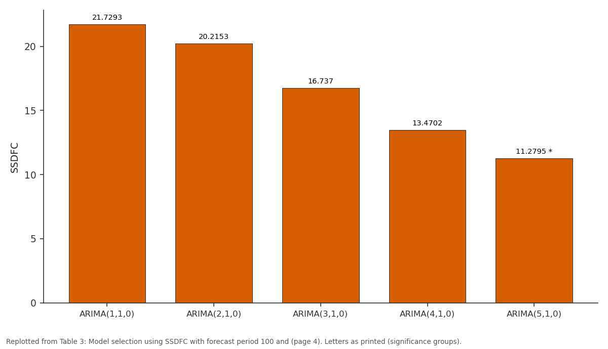
SSDFC: ARIMA(1,1,0) vs ARIMA(2,1,0) vs ARIMA(3,1,0) vs ARIMA(4,1,0) vs ARIMA(5,1,0)
Replotted from Table 3 (page 4) of the original paper. Every bar is the paper's own table value.
View source evidence ↗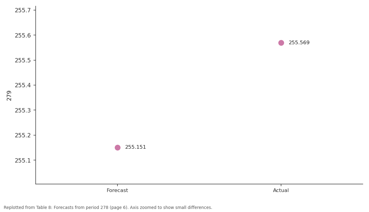
279: Forecast vs Actual
Replotted from Table 8 (page 6) of the original paper. Every bar is the paper's own table value.
View source evidence ↗Figures & tables
From the original paper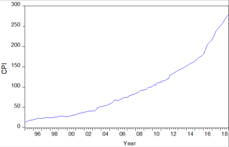 Figure 1
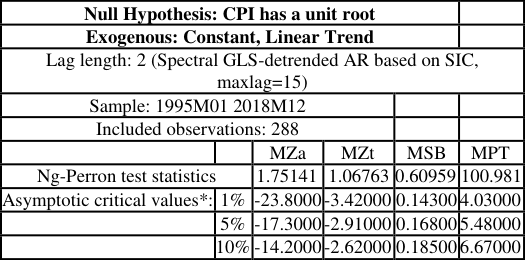 Table 1
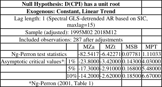 Table 2
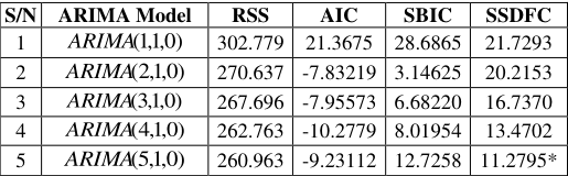 Table 3
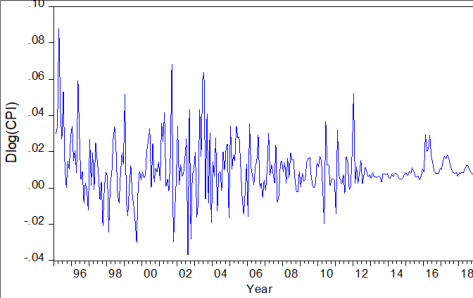 Figure 2
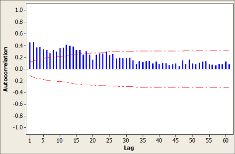 Figure 3
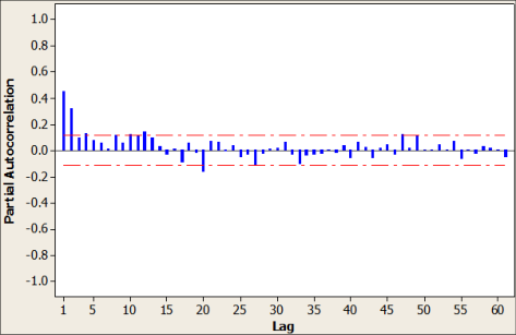 Figure 4
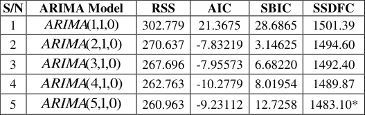 Table 4
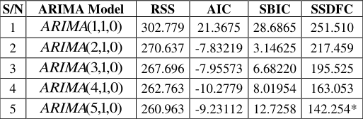 Table 5
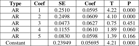 Table 6
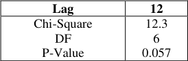 Table 7
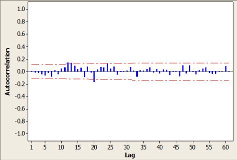 Figure 5
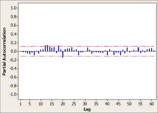 Figure 6
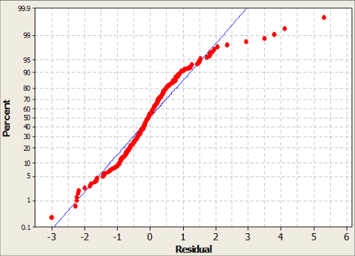 Figure 7
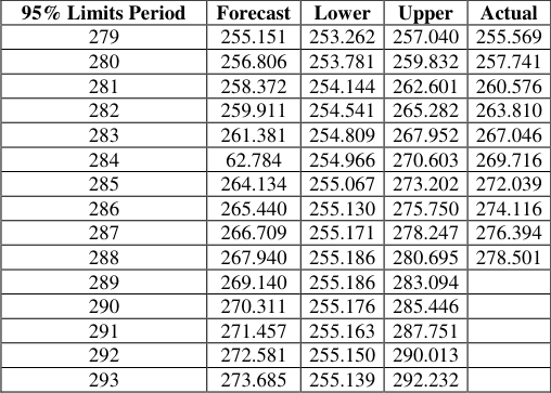 Table 8
Introduction
Consumer price index is a good and conventional measure of inflation and one of the key indicators of economic performance of every monetary policy of any country. The Consumer Price Index (CPI) measures the changes over time in the price level of consumer goods and services generally purchased by households. The year-on-year rate of change in the CPI is widely used as an indicator of the inflation affecting consumers. So any model that patterns the behaviour of CPI to its closest precision is very important to economic policy makers in forecasting future CPI. Habimana et al. (2016) [6] in their study employed Box and Jenkins methodology to model the dynamic of CPI and to forecast its future values in the short term in Rwanda. Applying main steps; model identification, parameter estimation and diagnostic checking, ARIMA (4,1,6) was selected as a potential model which can fits well data, as well as to make also accurate forecast. Hence, the forecast was made for 12 months ahead of the year 2016, and the findings have shown that the CPI was likely to continue rising up with time. Jere et al. (2016) [7] used monthly CPI data which were collected from January 2003 to December 2017 to model CPI in Zambia. The models that were compared are the Autoregressive Integrated Moving average (ARIMA) model and Multi-cointegration (ECM) model. Results showed that the ECM was the best fit model of CPI in Zambia since it showed smallest errors measures. Lastly, a forecast was done using the ECM and results show an average growth rate for food CPI at 6.63% and an average growth rate for non-food CPI at 7.41%. Nyoni (2019) [10] adopted Box and Jenkins approach in forecasting Australian CPI using ARIMA models. The result presented ARIMA (1, 1, 0) for forecasting CPI in Australia. The result of the study showed that CPI in Australia is likely to continue in an upward trend in the next decade. Kharimah et al (2015) [8] analyzed the CPI in Malaysia using ARIMA models with a data set ranging over the period January 2009 to December 2013 and revealed that the ARIMA(1, 1, 0) was the best model to forecast CPI in Malaysia. Sarangi et al (2018) [12] analyzed the consumer price index using Neural Network models with 159 data points and revealed that ANNs are better methods of forecasting CPI in India. Nyoni and Nathaniel (2019) [11] , based on ARMA, ARIMA and GARCH models; studied inflation in Nigeria using time series data on inflation http://www.mathsjournal.com rates from 1960 to 2016 and found out that the ARMA (1, 0, 2) model is the best model for forecasting inflation rates in Nigeria. Not understanding averagely the variability pattern of inflation in any economy can lead to miss targeted monetary policy. The effect of price instability due to inflationary pressure is inimical to the purchasing power of the national currency which culminates to high standards of living. Inflation reduces investment volume whether domestic and foreign investment in an economy. Forecasting CPI is an important factor for any economy because it is essential in economic planning for the future. Therefore, identifying a more accurate forecasting model is a major contribution to the economic growth of Nigeria.
Materials and Methods
This section presents methods and sources of data collection, variable measurement, and method of unit root test, ARIMA model specification, and model identification, method of data analysis, model comparison techniques and diagnostic checks.
Source of Data and variable measurement
The monthly consumer price index (CPI) data was obtained from published central bank of Nigeria (CBN, 2018) statistical bulletin. The univariate time series data collected covered the period of 1995M1-2018M12 (288 observations of monthly CPI data). CPI is usually a conventional measured inflation.
Moving Average (MA) Process
Moving average model is a sub-class of ARIMA models that uses lagged error term as predictor variable. Let . Then the q th order MA model is given as:
(1) 4This model is expressed in terms of past errors and estimated coefficients ) , ,
of the model are used for forecasting. Therefore only q errors predictors will affect the current level t x but higher order errors predictors do not affect t
x . Hence it is a short memory model.
Auto-Regression (AR) Process
An autoregressive model of order p, That is, AR (p) can be expressed as;
In this case, all previous values will have cumulative effects on the current level t x and thus, it is a long-run memory model.
ARMA (p, q) Model Specification
An integrated order one time series t X is said to follow an autoregressive moving average model of orders p and q denoted by ARMA(p, q) if it satisfies the difference equation
x is the original series, is the mean of the series,
. For L denotes the backshift operator defined by
and t u is the shock at time t, then Equation ( 4) can be rewritten as presented in Equation ( 4) below;
The process is stationary if, with stochastic initial conditionsthe stability conditions of the AR term are fulfilled, i.e. if ) (L A only has roots that are larger than 1 in absolute value.
If, If the time series t X is nonstationarity due to the presence of one or several of five conditions: outliers, random walk, drift, trend, or changing variance, it is conventional that first or second differencing (d) is necessary to achieve stationarity. Hence, the original series is said to follow an autoregressive integrated moving average model or orders p, d and q denoted by ARIMA (p, d, q). For nonstattionary series, Equation ( 6) can be of the form
Estimation of ARIMA (P, D, Q)
The ARIMA model estimation can be performed using either the method of maximum likelihood estimator or conditional least squares.
Method of maximum likelihood
Estimation of ARIMA model is often performed by exact maximize likelihood assuming Gaussian innovations. The exact Gaussian likelihood function for an ARIMA model is given by
where is the symmetric Toeplitz covariance matrix for the T draws from the ARMA process for the unconditional residuals (Doornik and Ooms 2003) [4] . The Kalman filter can be used to efficiently evaluate the likelihood. The Kalman filter works with the state space prediction error decomposition form of the likelihood, which eliminates the need to invert the large matrix . See Box, Jenkins, and Reinsel (2008, 7.4, p. 275) [3] for detail discussion.
Conditional least squares (CLS)
Box, Jenkins, and Reinsel (2008, Section 7.1.2 p 232.) point out that conditional on pre-sample values for the AR and MA errors, the normal conditional likelihood function may be maximized by minimizing the sum of squares of the innovations.
Notice that the conditional likelihood function depends on the data and the mean and ARIMA parameters only through the conditional least squares function d S ,
, , so that the conditional likelihood may be maximized by minimizing
. The coefficients are estimated using an iterative algorithm that calculates least squares estimates. At each iteration, the back forecasts are computed and SSE is calculated. For more details
Model identification
The ACF of an MA (q) model cuts off after lag q whereas that of an AR (p) model is a combination of sinusoidals dying off slowly. On the other hand, the PACF of an MA (q) model dies off slowly whereas that of an AR (p) model cuts off after lag p. The AR and MA models are known to exhibit some duality relationships. Parametric parsimony consideration in model building entails the use of the mixed ARMA fit in preference to either the pure AR or the pure MA fit.
Model Comparison
There are several model selection criteria in literature such as; Schwarz Bayesian information criterion (SBIC), Aikaike information criterion (AIC), residual sum of squares and so on. If n is the sample size and RSS is the residual sum of squares, then, SBIC and AIC are given as follows;
Where, n is the sample size, k is the number of estimated parameters (for the case of regression, k is the number of regressors) and RSS is the residual sum of squares based on the estimated model. However, it is good to note that both Schwarz Bayesian information criterion (SBIC) and AIC are affected by the number of parameters included to be estimated in a model. For the case of BIC, it penalizes free parameters while AIC becomes smaller as number of free parameters to be estimated increases. But for this study, sum of squares deviation forecast criterion introduced by Amaefula (2011) [1] will be used for model selection. And it is of the form;
Where l is the lead time, m is the number of forecast values to be deviated from the actual values (m should be reasonably large),
Ng and perron (NP) Test
Ng and Perron (2001) [9] constructed four statistics that are based upon the GLS detrended data d t y . These test statistics are modified forms of Philips and Perron z and t z statistics, the Bhargava (1986) [2] 1 R statistics, and the Elliot, Rothenberg, and Stock Point Optimal (ERS) (1996) [5] statistics. First, given the term;
The modified statistics may then be written as
, is the estimate from the auxiliary regression of equation ( 38) and
Note that NP test requires a specification for 𝑥t a choice of method estimating 𝑓0.
Data Analysis and Results
This The time series plot of CPI in Figure1 above exhibits a consistent upward trend for the period under study The plot of the first natural log difference in Figure2 above shows changes in CPI. It is observable that there are more variations in the first half of the series than in the second half of the series. And 2012 to 2018 the observable changes are centred around zero
NP Unit Root Test
In order to check the order of integration of the variables under study, NP unit root tests was carried out and the result are presented in Table1and 2 below; The Ng-Perron test statistics are all greater than 1%, 5% and 10% critical values, hence, the CPI is integrated order one (I( 1)) at its level series. This implies that the CPI is not stationary at the level series. The Ng-Perron test statistics in Table 2 are all less than 1%, 5% and 10% critical values, hence, the CPI at its first difference is integrated order zero (I (0)). This implies that the CPI is stationary at the first difference.
| Null Hypothesis: D(CPI) has a unit root | — | — | — | — | — |
|---|---|---|---|---|---|
| Exogenous: Constant, Linear Trend | |||||
| Lag length: 1 (Spectral GLS-detrended AR based on SIC, maxlag=15) | |||||
| Sample (adjusted): 1995M02 2018M12 | |||||
| Included observations: 287 after adjustments | |||||
| MZa | MZt | MSB | MPT | ||
| Ng-Perron test statistics | -82.5417 | -6.42271 | 0.07781 | 1.11033 | |
| Asymptotic critical values*: | 1% | -23.8000 | -3.42000 | 0.14300 | 4.03000 |
| 5% | -17.3000 | -2.91000 | 0.16800 | 5.48000 | |
| 10% | -14.2000 | -2.62000 | 0.18500 | 6.67000 | |
| *Ng-Perron (2001, Table 1) |
Table text extracted from the original PDF; superscript letters are shown inline. The original table image is below.
View original table image
Correlogram
The correlogram presents the plots of autocorrelation function (ACF) and the partial autocorrelation function (PACF) of first difference in CPI variable for model identification as presented in Figure3 and Figure4. The result of ACF in Figure3 shows a combination of sinusoidals dying off slowly. On the other hand, the PACF in Figure4 above cuts off after lag 2 thus, indicating that CPI follows an ARIMA (2, 1, 0) process. This tentative model identified will be compared with other possible ARIMA (p, d, q) models. The result of ACF in Figure3 shows a combination of sinusoidals dying off slowly. On the other hand, the PACF in Figure4 above cuts off after lag 2 thus, indicating that CPI follows an ARIMA (2,1,0) process. This tentative model identified will be compared with other possible ARIMA (p, d, q) models.
Model Comparison
This section presents compared 5 possible ARIM (p, 1, 0) models using SSDFC as presented in Table3 -Table5 below; The result of the model estimate in Table 6 showed that the coefficients of AR (1) and AR (2) are significant under 5% level. The implication is that the stationary CPI at current time is influenced by its lag1 and 2 values (and since the frequency of the data is monthly), it indicates that CPI is influenced by its past one and two month values. The ACF and PACF of residuals in Figure5 and Figure6 for the CPI data show non-significant spikes (the spikes are within the confidence limits) indicating that the residuals are uncorrelated. Therefore, the ARIMA (5, 1, 0) model appears to fit well and can be used to make forecasts The Modified Box-Pierce (Ljung-Box) Chi-Square statistic in Table 7 is not significant under 5% up to 12 th lag indicating that the residuals of the fitted ARIMA (5, 1, 0) are not correlated. Hence the model is well specified and adequate.
| Type | Coef | SE | Coef | T | P |
|---|---|---|---|---|---|
| AR | 1 | 0.2510 | 0.0595 | 4.22 | 0.000 |
| AR | 2 | 0.2498 | 0.0609 | 4.10 | 0.000 |
| AR | 3 | 0.0473 | 0.0627 | 0.75 | 0.451 |
| AR | 4 | 0.1155 | 0.0610 | 1.89 | 0.060 |
| AR | 5 | 0.0830 | 0.0598 | 1.39 | 0.166 |
| Constant | 0.23949 | 0.05695 | 4.21 | 0.000 |
Table text extracted from the original PDF; superscript letters are shown inline. The original table image is below.
View original table image
Discussion of result
The monthly CPI variable in Nigeria is integrated order one in its level series as reported by NP test and integrated order zero (I (0)) after the first difference. Hence, D (CPI) variable is stationary. The integrated order of CPI in Nigeria agrees with that of Kharimah et al. (2015) [8] , Habimana et al. (2016) [6] , Jere et al. (2016) [7] and Nyoni (2019) [10] for Malaysia, Rwanda, Zambia and Australia respectively. The SSDFC used as model selection criterion preferred ARIMA (5, 1 0) model as the best performing model with respect to prediction. This selected model is supported by RSS, indicating that SSDFC can be useful criterion to validate the best fitted model amongst two or more subclasses of ARIMA models or its likelihood. The ARIMA (5, 1, 0) selected differs from that of Nyoni & Nathaniel (2019) [11] who fitted ARMA (1, 0, 2) model for inflation in Nigeria. Though, Nyoni and Nathaniel used different variable for inflation rather than CPI. The Modified Box-Pierce (Ljung-Box) Chi-Square statistic in Table 7 is not significant indicating that the residuals of the fitted ARIMA (5, 1, 0) model are not correlated up to the 12 th lag. The ACF and PACF of the model residuals in Figure 4 and Figure 5 respectively showed that the residuals are uncorrelated. The probability plot in Figure 6 reveals that the residuals are normally distributed; hence, the fitted model is adequate. And the forecast values of CPI exhibit a rising trend.
Conclusion
The Box and Jenkins ARIMA (p, d, q) process was used to model CPI in Nigeria. And five (5) different sub-classes (order) of ARIMA (5, 1, 0) models were identified and compared using model selection criterion, specifically the SSDFC introduced by Amaefula (2011) [1] . The model comparison showed that ARIMA (5, 1, 0) is preferred. This chosen model was also supported by RSS and all the diagnostic tests indicated that the model is adequate. The finding reveals that CPI is significantly influenced by its past one and two month values. And CPI in Nigeria showed an upwards trend over the forecast period. From the findings, it becomes imperative for policy makers to engage more on how to make monetary policies more proactive so as to fight such increase in inflation (CPI) as reflected in the forecasts. However, based on the output performance of the compared models, SSDFC revealed that ARIMA (5, 1, 0) is preferred and can be recommended for predicting the dynamics of CPI in Nigeria.
Figures and tables from the paper
| Null Hypothesis: CPI has a unit root | — | — | — | — | — |
|---|---|---|---|---|---|
| Exogenous: Constant, Linear Trend | |||||
| Lag length: 2 (Spectral GLS-detrended AR based on SIC, maxlag=15) | |||||
| Sample: 1995M01 2018M12 | |||||
| Included observations: 288 | |||||
| MZa | MZt | MSB | MPT | ||
| Ng-Perron test statistics | 1.75141 | 1.06763 | 0.60959 | 100.981 | |
| Asymptotic critical values*: | 1% | -23.8000 | -3.42000 | 0.14300 | 4.03000 |
| 5% | -17.3000 | -2.91000 | 0.16800 | 5.48000 | |
| 10% | -14.2000 | -2.62000 | 0.18500 | 6.67000 |
Table text extracted from the original PDF; superscript letters are shown inline. The original table image is below.
View original table image
| 95% Limits Period | Forecast | Lower | Upper | Actual |
|---|---|---|---|---|
| 279 | 255.151 | 253.262 | 257.040 | 255.569 |
| 280 | 256.806 | 253.781 | 259.832 | 257.741 |
| 281 | 258.372 | 254.144 | 262.601 | 260.576 |
| 282 | 259.911 | 254.541 | 265.282 | 263.810 |
| 283 | 261.381 | 254.809 | 267.952 | 267.046 |
| 284 | 62.784 | 254.966 | 270.603 | 269.716 |
| 285 | 264.134 | 255.067 | 273.202 | 272.039 |
| 286 | 265.440 | 255.130 | 275.750 | 274.116 |
| 287 | 266.709 | 255.171 | 278.247 | 276.394 |
| 288 | 267.940 | 255.186 | 280.695 | 278.501 |
| 289 | 269.140 | 255.186 | 283.094 | |
| 290 | 270.311 | 255.176 | 285.446 | |
| 291 | 271.457 | 255.163 | 287.751 | |
| 292 | 272.581 | 255.150 | 290.013 | |
| 293 | 273.685 | 255.139 | 292.232 |
Table text extracted from the original PDF; superscript letters are shown inline. The original table image is below.
View original table image
References
12 in the original paper- Amaefula CG. Optimal identification of subclass of autoregressive integrated moving average model using sum of square deviation forecasts criterion. International Journal of Statistics and System. 2011; 6(1):35-40.
- Bhargava A. "On the Theory of Testing for Unit Roots in Observed Time Series," Review of Economic Studies. 1986; 53(3):369-384.
- Box George EP, Jenkins Gwilym M, Gregory Reinsel C. Time Series Analysis: Forecasting and Control, Fourth Edition, Hoboken, New Jersey: John Wiley & Sons, 2008.
- Doornik Jurgen A, Marius Ooms. "Computational Aspects of Maximum Likelihood Estimation of Autoregressive Fractionally Integrated Moving Average Models," Computational Statistics & Data Analysis. 2003; 42:333-348.
- Elliott Graham, Thomas J. Rothenberg and James H. Stock. "Efficient Test for an Autoregressive Unit Root." Econometrical. 1996; 64(4):813-836.
- Habimana Norbert, Anthony Wanjoya, Anthony Waititu. Modeling and Forecasting Consumer Price Index (Case of Rwanda). American Journal of Theoretical and Applied Statistics. 2016; 5(3):101-107. doi: 10.11648/j.ajtas.20160503.14
- Jere S, Banda A, Chilyabanyama R, Moyo E. Modeling Consumer Price Index in Zambia: A Comparative Study between Multicointegration and Arima Approach. Open Journal of StatisticsArticle ID: 91965. 2019; 9(2):13. 10.4236/ojs.2019.92018
- Kharimah F, Usman M, Elfaki W, Elfaki FAM. Time Series Modelling and Forecasting of the Consumer Price Bandar Lampung, Sci. Int (Lahore). 2015; 27(5):41194624.
- Serena Ng, Perron. "Lag Length Selection and Construction of Unit Root Test with Good Size and Power," Econometrica. 2001; 69(6):1519-1554.
- Nyoni T. Forecasting Australian CPI using ARIMA models. MPRA. 2019; 92412:1-11, Available at:https://mpra.ub.unimuenchen.de/92412/1/MPRA_paper_92412.pdf
- Nyoni T, Nathaniel SP. Modeling Rates of Inflation in Nigeria: An Application of ARMA, ARIMA and GARCH models, Munich University Library -Munich Personal RePEc Archive (MPRA), 2019, 91351.
- Sarangi PK, Sinha D, Sinha S, Sharma M. Forecasting Consumer Price Index using Neural Networks models, Innovative Practices in Operations Management and Information Technology-Apeejay School of Management, 2018, 84-93.