
Research article · 2018 · Full text
International Journal of Statistics and Applied MathematicsProfit analysis of two unit poly wrapping system with preventive maintenance and Degradation
Volume 3(2) · Pages 118–121
Research areasReliability and Maintenance OptimizationFault Detection and Control SystemsQuality and Supply Management
Abstract
Author-writtenToday most of the industries and plants are multi units systems i.e. not single unit containing. Various industries and processing systems are assembly of a number of units. In this paper we study a Polythene packing industry having a system comprising of two units namely Wrapper (A) and Bundler (B) having Preventive Maintenance in unit (A) only before partial failure and which undergoes Degradation on Complete Failure is analyzed. The failure of system collectively depends upon failure of each individual unit. Two units system is widely used in a number of process industries and many more others in which one unit is more important than second one and requires a more attention, so we apply preventive maintenance. If that single unit fails then the whole system fails. Considering the importance of such units in system Gupta, V. K. has discussed behavior with perfect and imperfect switch-over of systems using RPGT. So keeping in view the importance of every single unit in whole of the system, in this paper we have analyzed Two Unit System under Preventive Maintenance in main unit before complete failure and Degradation after Complete Failure. The unit may further deteriorate each time, so ultimately there will be stage when the unit will be beyond repair or it may not be advisable to repair it further due to higher cost maintenance or loss of production. Taking into account all the possibilities and path probabilities a transition diagram of system is traced out. As most of the units follow exponential failure rate, hence failure rate of individual is taken exponential. If the server reports that unit is not repairable then it is replaced by a new one. Fuzzy logic can be applied to determine the unit’s working in full capacity or reduced capacity.
Summary
Source-checkedPlain-language reading of the full paper, prepared with AI and checked against the text. Each point links to the authors' own words.
Why it matters
- Modern industrial plants typically consist of multi-unit systems rather than single units, as most processing systems are assemblies of multiple units. View evidence ↗
- Two-unit systems are common in process industries, often featuring one unit that is more critical than the other and thus requires preventive maintenance. View evidence ↗
- In these systems, the failure of the critical unit leads to the failure of the entire system. View evidence ↗
The question
- The study aims to analyze a two-unit system that undergoes preventive maintenance in the main unit before complete failure and experiences degradation after a complete failure. View evidence ↗
What they did
- The research focuses on a polythene packing industry system consisting of two units: a Wrapper (A) and a Bundler (B). View evidence ↗
- The model assumes that the failure rates of the individual units follow an exponential distribution. View evidence ↗
- A transition diagram was developed to map the system's path probabilities and possible states. View evidence ↗
- Profit is analyzed using a function that subtracts server busy costs and per-visit costs from the mean revenue earning rate multiplied by system availability. View evidence ↗
What they found
- The system's profit function is highly sensitive to and directly influenced by the rate of repair. View evidence ↗
- For small failure rates, increasing the repair rate leads to a gradual change in the profit function. View evidence ↗
- The profit function increases when both the steady state availability and the replacement factor increase. View evidence ↗
What it means
- The authors conclude that replacing a faulty unit is more beneficial for profit optimization than performing successive repairs on a degraded unit. View evidence ↗
Visual summary
2 visualsIllustrations explain the paper; charts are replotted from the paper's own table values.
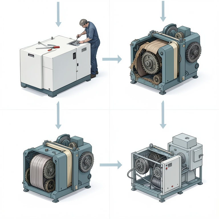
System State Transition Concept
AI-generated conceptual illustration (industrial poly wrapping machinery). It explains the idea and does not show study data.
View source evidence ↗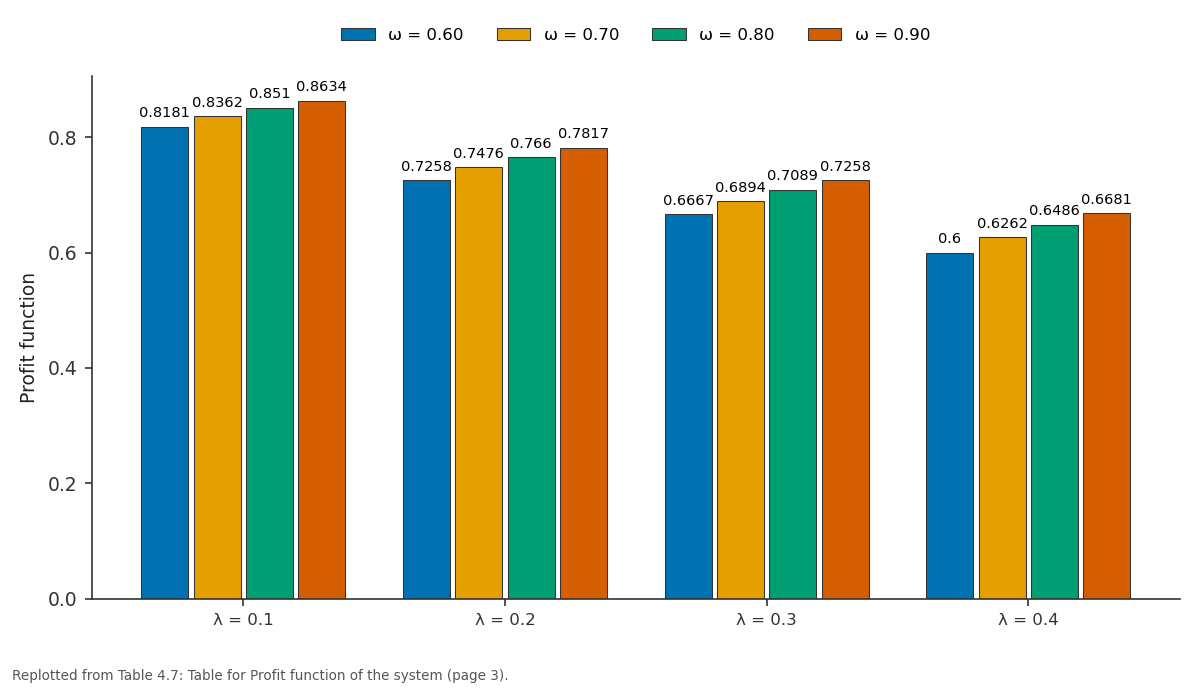
ω = 0.60 and ω = 0.70 and more: λ = 0.1 vs λ = 0.2 vs λ = 0.3 vs λ = 0.4
Replotted from Table 4 (page 3) of the original paper. Every bar is the paper's own table value.
View source evidence ↗Figures & tables
From the original paper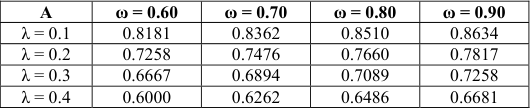 Table 4
Introduction
Assumptions: - Here we have discussed the system for long run means for time taken is infinite. Preventive Maintenance is available for main unit Wrapper (A) only not to other unit. And switching of units is perfect. After complete failure replacement facility is immediate.
There is single server facility. Repair of unit A is imperfect and repaired unit is not good as new one on complete failure i.e. system goes in degraded state after first complete failure. Considering the various possibilities and assumptions the transition diagram of the system is drawn as under Maths 2018; 3(2): 118-121 Dr. Vijay Goyal Assistant Professor of Mathematics, Manohar Memorial (PG) College, Fatehabad, Haryana, India SR Patel Assistant Professor of Mathematics, Manohar Memorial (PG) College, Fatehabad, Haryana, India Correspondence Dr.
Vijay Goyal Assistant Professor of Mathematics, Manohar Memorial (PG) College, Fatehabad, Haryana, India ,ଵ= λ1/(λ+λ1+λ4) ,ଶ= λ/(λ+λ1+λ4) ,= λ/(λ+λ1+λ4) Description of Model Initially the two units A and B are working in full capacity initially in state S0. The system can be in any of the following states with respect to the above symbols. States S0, S1, S3 and S4 are regenerative states. S0=AB, S1=ܣ̅B, S2=aB, S3=ܣ̅1B, S4=a1B, S5=ܣ̅1b, S6=ܣ̅b, S7=Ab Determination of base-state In the transition diagram there are four, two, two, four, three, one, one and one primary circuits at the vertices 0, 1, 2, 3, 4, 5, 6 & 7 respectively.
As there are four primary circuits associated each of the vertices 0&3. But secondary circuited is minimum in state 0 so state 0 is base state. Transition Probabilities qi,j(t) Pij = q*i,j(t) ݍ,ଵ= λ1݁ିሺఒభାఒାఒరሻ௧ ݍ,ଶ= λ݁ିሺఒభାఒାఒరሻ௧ ݍ,= λ4݁ିሺఒభାఒାఒరሻ௧ ݍଵ,= ݓଵ݁ିሺ௪భାఒమାఒరሻ௧ ݍଵ,ଶ= ߣଶ݁ିሺ௪భାఒమାఒరሻ௧ ݍଵ,= ߣସ݁ିሺ௪భାఒమାఒరሻ௧ ଵ,= w1/(w1+λ2+λ4) ଵ,ଶ= λ2/(w1+λ2+λ4) ଵ,= λ4/(w1+λ2+λ4) ݍଶ,ଷ= ݓଶ݁ି௪మ௧ ଶ,ଷ= w2/w2 = 1 ݍଷ,ସ= ߣଷ݁ିሺఒయశఒరሻ௧ ݍଷ,ହ= ߣସ݁ିሺఒయశఒరሻ௧ ଷ,ସ= λ3/(λ3+λ4) ଷ,ହ= λ4/(λ3+λ4) ݍସ,= ݃ሺݐሻ݁ି௪య௧ ݍସ,ଷ= ݓଷ݁ି௪య௧݃ሺݐሻ തതതതതത ସ,= g*w3 ସ,ଷ= 1-g*w3 ݍହ,ଷ= ݓସ݁ି௪ర௧ ହ,ଷ= w4/w4 = 1 ݍ,ଵ= ݓସ݁ି௪ర௧ ,ଵ= w4/w4 = 1 ݍ,= ݓସ݁ି௪ర௧ ,= w4/w4 = 1 Mean Sojourn Times Ri(t) µi=Ri*(0) ܴሺݐሻ= ݁ିሺఒభାఒାఒరሻ௧ µ0 = 1/(λ+λ1+λ4) ܴଵሺݐሻ= ݁ିሺ௪భାఒమାఒరሻ௧ µ1 = 1/(w1+λ2+λ4) ܴଶሺݐሻ= ݁ି௪మ௧ µ2 = 1/w2 ܴଷሺݐሻ= ݁ିሺఒయାఒరሻ௧ µ3 = 1/(λ3+λ4) ܴସሺݐሻ= ݁ି௪య௧݃ሺݐሻ തതതതതത µ4 = [1-g*[(w3)]/w3 ܴହሺݐሻ= ݁ି௪ర௧ µ5 = 1/w4 ܴሺݐሻ= ݁ି௪ర௧ µ6 = 1/w4 ܴሺݐሻ= ݁ି௪ర௧ µ7 = 1/w4 The path probabilities for the steady state are given w.r.t. Base State ‘0’ are V0,0 = {(0,1,0)/[1-(1,6,1)}+{(0,7,0)/1}+{(0,1,2,3,4,0)/[1-(1,6,1)1-(3,4,3)1-(3,5,3)}] +{(0,2,3,4,0)/[1-(3,5,3)[1-(3,4,3)}] = (p0,1p1,0)/(1-p1,6p6,1)+p0,7p7,0+(p0,1p1,2p2,3p3,4p4,0)/(1-p1,6p6,1)(1-p3,4 p4,3) (1-p3,5p5,3)+ (p0,2p2,3p3,4p4,0)/[(1-p3,4 p4,3)(1-p3,5p5,3)] =1 V0,1 = {p0,1/1-(1,6,1)} = {λ/(λ1+λ+λ4)}/1-λ4(λ2+w1+λ4) = {λ1(λ2+w1+λ4)/(λ2+w1) (λ1+λ+λ4)} V0,2 = {(0,1,2)/1-(1,6,1)}+(0,2) = {p0,1p1,2/1-p1,6p6,1}+ p0,2 = [{λ1/(λ1+λ+λ4)λ2/(λ2+w1+λ4)}/1-{λ4(w1+λ2+λ4)}]+{λ/(λ1+λ+λ4)} = {λ1λ2+λ(λ2+w1)}/(λ1+λ+λ4)(λ2+w1)} V0,3 = {(0,1,2,3)/1-(1,6,1)1-(3,5,3)1-(3,4,3)}+{(0,2,3)/1-(3,5,3)1-(3,4,3)} = {p0,1p1,2 p2,3/(1-p1,6p6,1)(1-p3,5p5,3)(1-p3,4 p4,3)}+{p0,2 p2,3/(1-p3,5p5,3)(1-p3,4 p4,3)} = {(λ3+λ4)2(λ1λ2+λλ2+λw1)/λ3λ4(λ1+λ+λ4)(λ2+w1)} V0,4 = {(0,1,2,3,4)/[1-(1,6,1)1-(3,5,3)1-(3,4,3)}+{(0,2,3,4)]/[1-(3,5,3)1-(3,4,3)} = {p0,1p1,2 p2,3p3,4/(1-p1,6p6,1)(1-p3,5p5,3)(1-p3,4 p4,3)}+{p0,2 p2,3p3,4/(1-p3,5p5,3) (1-p3,4 p4,3)} = {(λ3+λ4)/λ4(λ1+λ+λ4)}{(λ1λ2+λw1+λλ2)/(w1+λ2)} V0,5 = {(0,1,2,3,5)/1-(1,6,1)1-(3,5,3)1-(3,4,3)}+{(0,2,3,5)/1-(3,5,3)1-(3,4,3)} = {p0,1p1,2 p2,3p3,5/(1-p1,6p6,1)(1-p3,5p5,3)(1-p3,4 p4,3)}+{p0,2 p2,3p3,5/(1-p3,5p5,3) (1-p3,4 p4,3)} = {(λ3+λ4)/λ3(λ1+λ+λ4)}{(λ1λ2+λw1+λλ2)/(w1+λ2)} V0,6 = {(0,1,6)/1-(1,6,1)} = p0,1p1,6/(- p1,6 p6,1) = [{λ1/(λ1+λ+λ4)}{λ4/(w1+λ2+λ4)}]/ [1-{λ4/(w1+λ2+λ4)}] Evaluation of parameters of the system The reliability measures of the system (under steady state conditions) are evaluated by determining a ‘base-state’.
The parameter MTSF is determined w. r. t. the initial state ‘0’ and the other parameters are obtained by using base-state. (i). Mean Time to System Failure (MTSF) (T0) The regenerative un-failed states to which the system can transit (initial state ‘0’), before entering any failed state are: ‘i’ MTSF (T0) = =, 1, 2, 3, 4, 5, 6, 7 taking ‘ ’ = ‘0’. T0 = [(0,0)µ0+(0,1)µ1]/[1-(0,1,0) = (p0,0µ0+p0,1µ1)/(1-p0,1p1,0) = (λ2+λ4+w1+λ1)/[(λ1+λ+λ4)(w1+λ2+λ4)-λ1w1] (ii). Availability of the System The regenerative states at which the system is available are ‘j’ = 0, 1, 3 and the regenerative states are ‘i’ = 0 to 4 taking ‘ξ’ = ‘0’ the total fraction of time for which the system is available is given by A0 = ൣ∑ܸక, , ݂, ߤ൧ ൊ ൣ∑ܸక, , ݂, ߤ ଵ൧ =(V0,0µ0+V0,1µ1+V0,3µ3)(V0,0µ01 +V0,1µ11 +V0,2µ21+V0,3µ31+V0,4µ41+V0,5µ51+V0,6µ61 +V0,7µ71) = [{(λ2+w1)/1}+λ1+{(λ3+λ4)(λ1λ2+λw1+λλ2)/λ3λ4}]/[{λ2+w1+λ1(λ1λ2+λλ2+λw1)/w1} +{(λ3+λ4)(λ1λ2+λλ2+λw1)/λ3λ4}+{(λ3+λ4)(λ1λ2+λw1+λλ2)(1-g*(w3))/λ4w3} +{(λ3+λ4)(λ1λ2+λw1+λλ2)/λ3w4}+{λ1λ4/w4}+{λ4(λ2+w1)/ w4}] (iii).
Proportional Busy Period of the Server B0 = ൣ∑ܸక, , ݊൧ ൊ ൣ∑ܸక, , ߤ ଵ൧ =(V0,1µ1+V0,2µ2+V0,4µ4+V0,5µ5+V0,6µ6+V0,7µ7)/(V0,0µ0 +V0,1µ1+V0,2µ2+V0,3µ3 +V0,4 µ4 +V0,5 µ5+V0,6µ6+V0,7µ7) = [(λ1/1)+(λ1λ2+λλ2+λw1)/w2}+{(λ3+λ4)(λ1λ2+λλ2+λw1)(1-g*w3)/λ4w3}+{(λ3+λ4) (λ1λ2+λλ2+λw1)/λ3λ4}+{λ1λ4/w4}+{λ1(λ2+w1)/w4}]/[{(λ2+w1)+λ1(λ1λ2+λλ2+λw1) /w2}+{(λ3+λ4)(λ1λ2+λλ2+λw1)/λ4w3}+{(λ3+λ4)(λ1λ2+λλ2+λw1) (1-g*w3)/λ3w4} +{(λ3+λ4)(λ1λ2+λλ2+λw1)/λ4w3}+{λ1λ4/w4}{λ4(λ2+w1)/w4}] Profit function of the system Profit analysis of the system can be done by using the profit function P0 = Mean Revenue Earning Rate *Availability of the system - mean server cost that server is busy *total busy period - mean cost per visit which the server charges *number of visits server called in a unit time. P0 = C1A0 – C2B0 – C3V0 =C1[{(λ2+w1)/1}+λ1+{(λ3+λ4)(λ1λ2+λw1+λλ2)/λ3λ4}]/[{λ2+w1+λ1(λ1λ2+λλ2+λw1)/w1}+ {(λ3+λ4)(λ1λ2+λλ2+λw1)/λ3λ4}+{(λ3+λ4)(λ1λ2+λw1+λλ2)(1-g*(w3))/λ4w3}+{(λ3+λ4) (λ1λ2+λw1+λλ2)/λ3w4}+{λ1λ4/w4}+{λ4(λ2+w1)/ w4}] = [{(λ2+w1)/1}+λ1+{(λ3+λ4)(λ1λ2+λw1+λλ2)/λ3λ4}]/[{λ2+w1+λ1(λ1λ2+λλ2+λw1)/w1} +{(λ3+λ4)(λ1λ2+λλ2+λw1)/λ3λ4}+{(λ3+λ4)(λ1λ2+λw1+λλ2)(1-g*(w3))/λ4w3} +{(λ3+λ4)(λ1λ2+λw1+λλ2)/λ3w4}+{λ1λ4/w4}+{λ4(λ2+w1)/ w4}] Particular Cases Now we discuss special cases when λi = λ for i = 1, 2, 4 and wi = w, i = 1, 2, 4 and repair rate after degradation is given by recurrence relation. λn = (1+α)λn-1 MTSF (T0) = (3λ+w)/[{3λ/(2λ+w)-λw} = (3λ+w)/(6λ2+2λw) = 1/2λ dT0/dλ = -1/2λ2 < 0 i.e. MTSF decreases with increases in failure rate λ. Profit Function = P0 [(λ+w)+λ+2(2λ+w)]/[(2λ+w)+{λ(2λ+w)/w}+(4λ+w)+(6λ+w) +{2(2λ2+λw)/w}{w/(r+w)}+{(4λ2+2λw)/w}+{λ2/w}{λ(λ+w)/w}] = [12λw+6w2]/ [22λw+6w2+4λ2] Table 4.7: Table for Profit function of the system A ω = 0.60 ω = 0.70 ω = 0.80 ω = 0.90 λ = 0.1 0.8181 0.8362 0.8510 0.8634 λ = 0.2 0.7258 0.7476 0.7660 0.7817 λ = 0.3 0.6667 0.6894 0.7089 0.7258 λ = 0.4 0.6000 0.6262 0.6486 0.6681 Profit function Graph for Different Repair Rates
| A | ω = 0.60 | ω = 0.70 | ω = 0.80 | ω = 0.90 |
|---|---|---|---|---|
| λ = 0.1 | 0.8181 | 0.8362 | 0.8510 | 0.8634 |
| λ = 0.2 | 0.7258 | 0.7476 | 0.7660 | 0.7817 |
| λ = 0.3 | 0.6667 | 0.6894 | 0.7089 | 0.7258 |
| λ = 0.4 | 0.6000 | 0.6262 | 0.6486 | 0.6681 |
Table text extracted from the original PDF; superscript letters are shown inline. The original table image is below.
View original table image
Result
Discussion and Conclusions: In present time, competitions between different industries have increased demands on production systems. Customer satisfaction or reliability of a brand depends upon the production system’s capability to provide goods and services on time and meeting the required quality specification. To fulfill the customer’s requirement, the system must be reachable. Here we have studied the system for maximization of net profit and obtained that it is independent of base state and mean time to system failure.
We have seen that profit function is directly influenced by repair rate and highly sensitive to rate of repair. As repair rate is increased then profit function have gradual change for small values of failure rates. Also we see that if study state availability increases and replacement factor increases then also profit function increases. Hence, we conclude that for optimization of profit replacement of faulty unit is more beneficial then successive repairs of degraded unit.
References
6 in the original paper- Gupta VK. Analysis of a single unit system using a base state. Aryabhatta J of Maths & Info. 2011; 3 (1):59-66.
- Goel P, Singh J. Availability Analysis of A Chemical Plant Having Two Imperfect Switch Over Devices; Proc. (Reviewed) Conference On Mathematics And Its Application In Engg. And Industry, 1996, 138-144.
- Gupta P, Sharma SK, Goyal A, Vikas. Performance Analysis of The Yarn Production Subsystem A Part Of Carded Yarn Manufacturing Plant-A Case Study. Journal of Mathematics and Systems Science (JMASS). 2009; 5(2):58-63.
- Kishor A, Yadav SP, Kumar S. A Fuzzifying Approach to Stochastic Programming. Operational Research Society of India. 2009; 50(3):214-224.
- Gupta VK, Singh J, Kumar K, Goel P. Profit Analysis of a q Single Unit Operating System with a Capacity Factor and Undergoing Degradation. Journal of Mathematics & System Sciences. 2009; 5(2):129-142. ISSN 0975-7139
- Singh J. Reliability Technology In Daily Life. Journal of Mathematics and Systems Science (JMASS). 2011; 7(1):54-58.