
Research article · 2017 · Full text
International Journal of Statistics and Applied MathematicsA stochastic modeling for paddy production in Tamilnadu
Volume 2(5) · Pages 14–21
Research areasAgricultural Economics and Practices
Abstract
Author-writtenThis paper investigates predictive performance of time series analysis method for paddy production trends in Tamilnadu. In the present study had been carried out on the basis of time-series production data of paddy crop pertaining to the period 1960 to 2015 had been collected and forecasting the production for 2016 to 2020 using ARIMA (Autor Regressive Integrated Moving Average), Simple exponential smoothing, Brown exponential smoothing and Damped exponential smoothing models.
Summary
Source-checkedPlain-language reading of the full paper, prepared with AI and checked against the text. Each point links to the authors' own words.
Why it matters
- Agriculture is a critical component of the Indian economy, employing 54.6% of the population as of the 2011 census. View evidence ↗
- Tamil Nadu is currently the second largest producer of rice in India. View evidence ↗
- Timely forecasting of paddy production is essential for planning strategies to increase crop yields. View evidence ↗
The question
- The study aims to identify the most appropriate model for forecasting paddy production in Tamil Nadu by comparing various smoothing techniques and ARIMA time series modeling. View evidence ↗
What they did
- The researchers used time-series production data for paddy crops in Tamil Nadu collected from 1960 to 2015. View evidence ↗
- Production for the years 2016 to 2020 was forecasted using ARIMA, Simple exponential smoothing, Brown exponential smoothing, and Damped exponential smoothing models. View evidence ↗
- The SPSS software package was employed to estimate model parameters and calculate related statistics. View evidence ↗
What they found
- Analysis of the time plot for milled rice production from 1960 to 2015 showed an increasing trend. View evidence ↗
- Among the smoothing techniques, Brown's exponential smoothing was most appropriate, with a minimum mean absolute percentage error of 7.787 at α= 0.214. View evidence ↗
- The ARIMA (0,1,1) model was the most effective ARIMA model, explaining 95% of the variation in the data series (R² = 0.95). View evidence ↗
- When comparing all smoothing techniques, Holt's winter smoothing was found to be superior to the others. View evidence ↗
What it means
- The authors conclude that Holt's winter smoothing and the ARIMA (0,1,1) model are the most appropriate for forecasting paddy production. View evidence ↗
- The authors suggest preferring the Holt's winter model because it is non-parametric and does not require the verification of stationary conditions, unlike ARIMA models. View evidence ↗
Visual summary
3 visualsIllustrations explain the paper; charts are replotted from the paper's own table values.
Forecasting Model Comparison Workflow
AI-generated conceptual illustration (paddy plants in a field). It explains the idea and does not show study data.
View source evidence ↗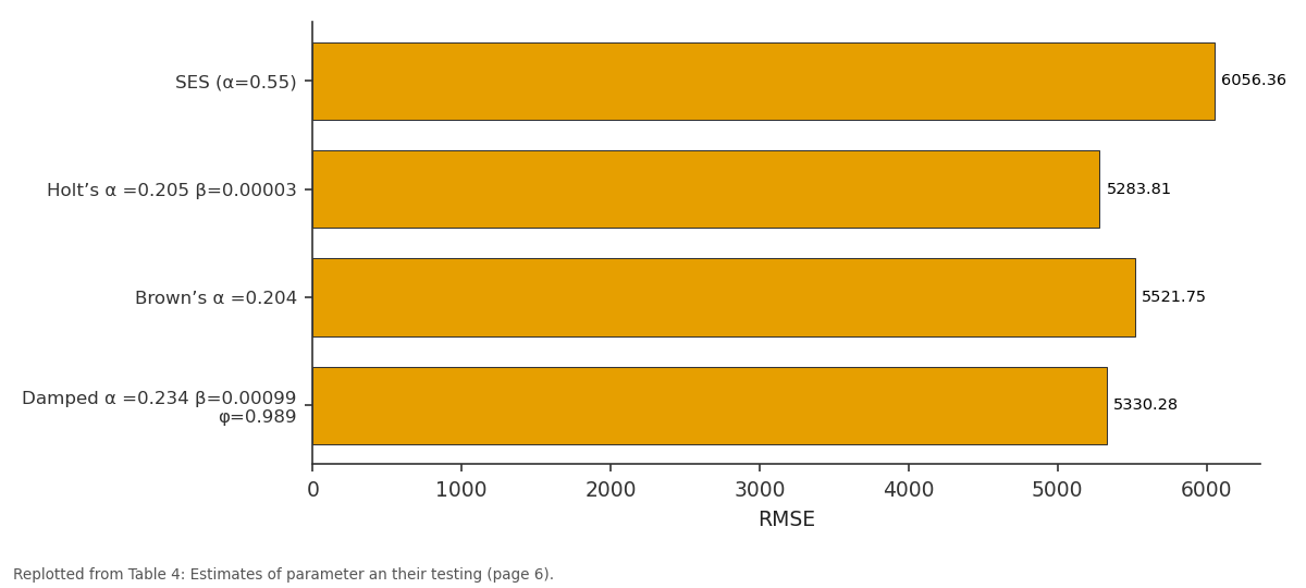
RMSE: SES (α=0.55) vs Holt’s α =0.205... vs Brown’s α =0.204 vs Damped α =0.234...
Replotted from Table 4 (page 6) of the original paper. Every bar is the paper's own table value.
View source evidence ↗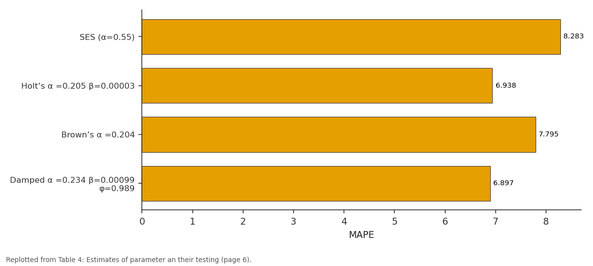
MAPE: SES (α=0.55) vs Holt’s α =0.205... vs Brown’s α =0.204 vs Damped α =0.234...
Replotted from Table 4 (page 6) of the original paper. Every bar is the paper's own table value.
View source evidence ↗Figures & tables
From the original paper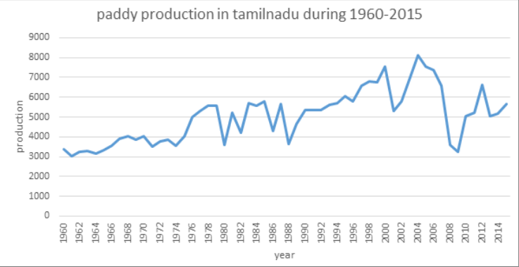 Figure 1
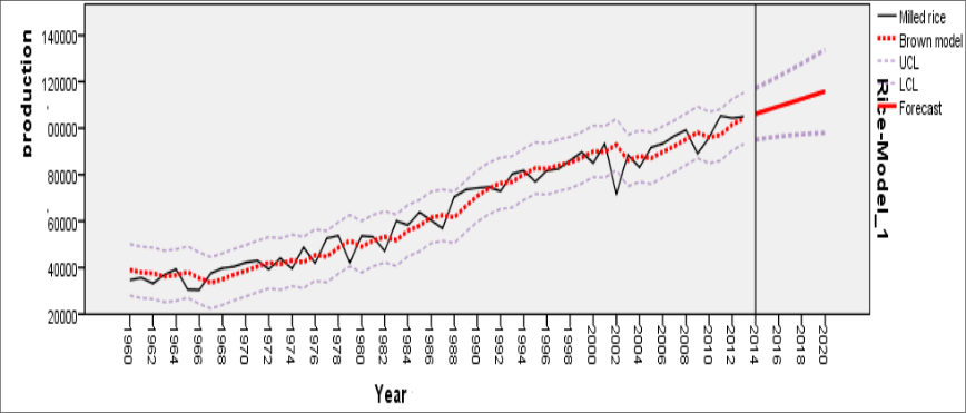 Figure 2
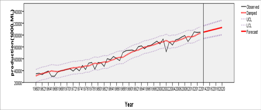 Figure 3
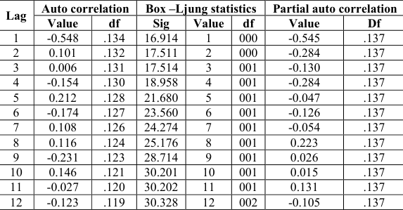 Table 1
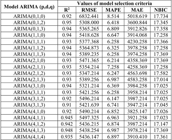 Table 2
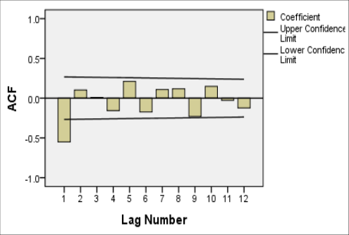 Figure 4
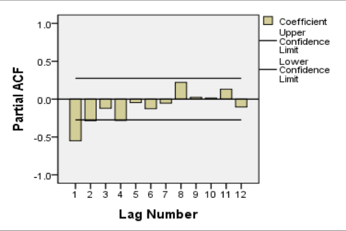 Figure 4
 Table 3
 Table 4
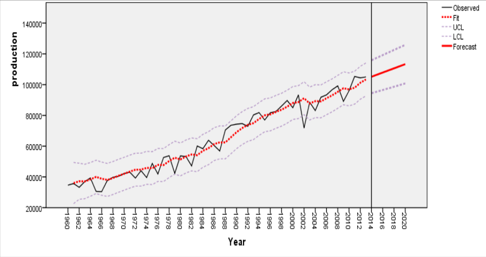 Figure 5
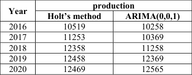 Table 5
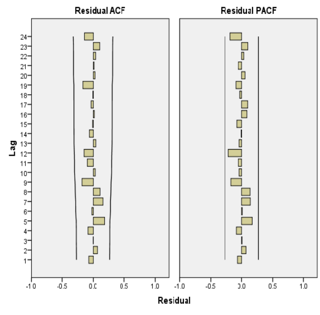 Figure 6
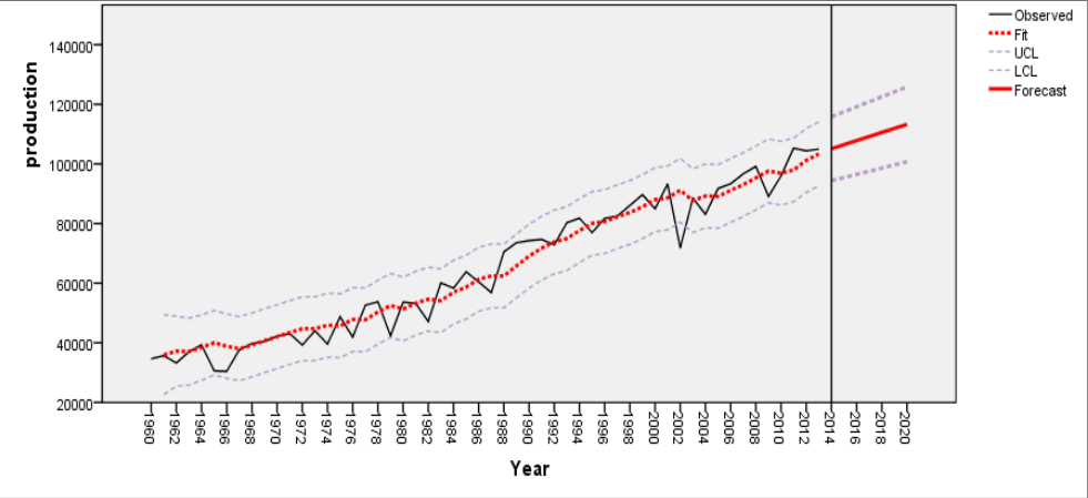 Figure 7
Introduction
Agriculture plays a vital role in India's economy. 54.6% of the population is engaged in agriculture and allied activities (census 2011).Tamil Nadu has historically been an agricultural state, while its advances in other fields launched the state into competition with other areas. Agriculture is heavily dependent on the river water and monsoon rains. Tamil Nadu is also the leading producer of kambu, corn, rye, groundnut, oil seeds and sugarcane in India. At present, Tamil Nadu is India's second biggest producer of rice. Agriculture continues to be the most predominant sector of the State economy, as 70 percent of the population is engaged in Agriculture and allied activities for their livelihood. Tamil Nadu has all along been one of the states with a creditable performance in agricultural production with the farmers relatively more responsive and receptive to changing technologies and market forces. Heavy consumption of this food crop has become an important issue the yield of rice of our Country. Considering these facts in mind it is very important to have timely forecast of this crop in Order to plan the strategies to increase the yield. To make the best forecast of paddy production in India, appropriate time series forecasting Methods are discussed by Makridakis and Hibbon (1979), Pankratz (1983), Granger and Newbold (1986), Makridakis et al. (1998).One of the most successful time series forecasting techniques is Box-Jenkin type ARIMA model is given by Box and Jenkins (1970) which is the most commonly used linear statistical model. Accordingly the present study was aims to find appropriate model for forecasting paddy production in tamilnadu based on different smoothing techniques and ARIMA time series modelling and to select more appropriate forecasting model based on model selection criteria.
Materials
In the present study had been carried out on the basis of time-series production data of paddy Crop pertaining to the period 1960 to 2015 had been collected in Tamil Nadu from the official Website (http://www.indianmundi.com) and forecasting the production for 2016 to 2020 using ARIMA (Auto Regressive Integrated Moving Average), Brown exponential smoothing and Damped exponential smoothing models. SPSS package was used to estimate the model Parameters and all other related statistics.
Methods
After ensuring the presence of trend in the data, smoothing of the data is the next requirement for time series analysis. For smoothing the common techniques discussed by Gardner (1985) are simple Exponential smoothing (SES), Holt's linear exponential smoothing (LES), Additive Holt's model with a damping factor, brown's exponential smoothing. All these smoothing techniques have been employed to paddy production data set. Among these smoothing techniques, best one has been identified based on model selection criteria. ARIMA model also was employed and compared with the smoothing techniques. The computational procedures are discussed in detail in sequence below.
Simple exponential smoothing.
The simplest of the exponentially smoothing methods is naturally called "simple exponential smoothing" (SES). (In some books, it is called "single exponential smoothing".) This method is suitable for forecasting data with no trend or seasonal pattern. Using the naïve method, all forecasts for the future are equal to the last observed value of the series, / = for h=1,2,…. Hence, the naïve method assumes that the most current observation is the only important one and all previous observations provide no information for the future. This can be thought of as a weighted average where all the weight is given to the last observation. Using the average method, all future forecasts are equal to a simple average of the observed data,
for h=1,2,…. Hence, the average method assumes that all observations are of equal importance and they are given equal weight when generating forecasts. We often want something between these two extremes. For example it may be sensible to attach larger weights to more recent observations than to observations from the distant past. This is exactly the concept behind simple exponential smoothing. Forecasts are calculated using weighted averages where the weights decrease exponentially as observations come from further in the past ---the smallest weights are associated with the oldest observations:
Where 0≤α≤1 is the smoothing parameter. The one-stepahead forecast for time T+1 is a weighted average of all the observations in the series y1,…,Yt. The rate at which the weights decrease is controlled by the parameter α.
Let an observed time series be y1,y2,….yn. Formally, the simple exponential smoothing equation takes the form of
Where is the actual, known series value for time period T, is the forecast value of the variable Y for time period T, is the forecast value for time period T +1 and α is thesmoothing constant is given by Brown et al.(1961). The forecast is based on weighting the most recent observation with a weight α and weighting the most recent forecast with a weight of 1-α.
Holt's exponential smoothing Holt (2004) extended simple exponential smoothing to allow forecasting of data with a trend. This method involves a forecast equation and two smoothing equation
where t,bt denotes an estimate of the level of the series at time t, bt denotes an estimate of the trend (slope) of the series at time tt, αα is the smoothing parameter for the level, 0≤α≤1 and β * is the smoothing parameter for the trend, 0≤β * ≤1.
Brown's exponential smoothing
Brown's exponential smoothing is given by Brown (1961).
The smoothing equations are
The h step ahead prediction equation is = + ((ℎ -1) + 1/ ) .
Damped exponential smoothing
The h-step-ahead prediction equation is
This is, you forecast y h-steps ahead by taking the last available estimated level state and multiplying the last available trend (slope), Tt, with ϕ i = dampening factor.
ARIMA Model
A time series is a set of numbers that measures the status of some activity over time. It is the historical record of some activity, with measurements taken at equally spaced intervals with a consistency in the activity and the method of measurement.
Moving Average Process
Moving average models were first considered by Slutsky (1927) and Wold (1938). The Moving Average Series can be written as
We call such a series a moving average of order q and abbreviate the name to MA (q). Where, Y is the original series and e is the series of errors
Auto-Regressive Process
Yule (1926) carried out the original work on autoregressive processes. Autoregressive processes are as their name suggests regressions on themselves. Specifically, a p th -order autoregressive process { } satisfies the equation
The current value of the series is a linear combination of the most recent past values of itself plus an "innovation" term that incorporates everything new in the series at time that is not explained by the past values. Thus, for every , we assume that is independent of , , ⋯ .
Autoregressive Integrated Moving Average (ARMIA) model
The Box and Jenkins (1970) procedure is the milestone of the modern approach to time series analysis. Given an observed time series, the aim of the Box and Jenkins procedure is to build an ARIMA model. In particular, passing by opportune preliminary transformations of the data, the procedure focuses on Stationary processes. In this study, it is tried to fit the Box-Jenkins Autoregressive Integrated Moving Average (ARIMA) model. This model is the generalized model of the nonstationary ARMA model denoted by ARMA (p, q) can be written as
Where, is the original series, for every , we assume that is independent of + + + ⋯ + .A time series { } is said to follow an integrated autoregressive moving average (ARIMA) model if the d th difference = is a stationary ARMA process. If { } follows an ARMA (p, q) model, we say that { }is an ARIMA (p, p, q) process. Fortunately, for practical purposes, we can usually take d = 1 or at most 2. Consider then an ARIMA (p, 1, q) process. With =we have
Box and Jenkins procedures 1. Preliminary analysis: create conditions such that the data at hand can be considered as the realization of a stationary stochastic process. 2. Identification: specify the orders p, d, q of the ARIMA model so that it is clear the number of parameters to estimate. Recognizing the behavior of empirical autocorrelation functions plays an extremely important role. 3. Estimate: efficient, consistent, sufficient estimate of the parameters of the ARIMA model (maximum likelihood estimator). 4. Diagnostics: check if the model is a good one using tests on the parameters and residuals of the model. Note that also when the model is rejected, still this is a very useful step to obtain information to improve the model.
Usage of the model: if the model passes the diagnostics
step, then it can be used to interpret a phenomenon, forecast.
Jarque-Bera Test
We can check the normality assumption using Jarque-Bera (1978) test, which is a goodness of fit measure of departure from normality, based on the sample kurtosis (k) and Skewness(s). The test statistics Jarque-Bera (JB) is defined as
Where n is the number of observations and k is the number of estimated parameters. The statistic JB has an asymptotic chisquare distribution with 2 degrees of freedom, and can be used to test the hypothesis of Skewness being zero and excess kurtosis being zero, since sample from a normal distribution have expected Skewness of Zero and expected excess kurtosis of zero.
Ljung-Box test
Ljung-Box Test can be used to check autocorrelation among the residuals. If a model fit well, the residuals should not be correlated and the correlation should be small. In this case the null hypothesis is
Where, N is the no of observation used to estimate the model. This statistic Q* approximately follows the chi-square distribution with ( -) df, where q is the no of parameter should be estimated in the model. If Q* is large (Significantly large from zero), it is said that the residuals autocorrelation are as a set are significantly different from zero and random shocks of estimated model are probably auto-correlated. So one should then consider reformulating the model.
Model Performance Measures
The following measures have been used to study the different model performance.
Root Mean Square Error (RMSE) =
Root Mean Square Error (RMSE) =
∑ (
Where is the original paddy production in different years and is the forecasted paddy production in the corresponding years and n is the number of years used as forecasting period. NBIC(p,q)=In v*( , ) + ( + ) ( ) ;Where p and q are the order of AR and MA processes respectively and n is the number of observations in the time series and v* is the estimate of white noise variance .
Results and discussion
Exponential Smoothing Linear model: Time plot (Fig. 1) of milled rice production data revealed that there is increased trend in the data period 1960-2015. For smoothing of the data, Brown's exponential smoothing technique was found to be most appropriate. Various combinations of Level and Trend based on range between 0.1 to 0.9 with increments of 0.1 were tried and mean absolute percentage error ( 7.787) was least for α= 0.214 (Fig. 2 and Table 4). Damped exponential smoothing technique was found to be most appropriate. Various combinations of Level and Trend based on range between 0.1 to 0.9 with increments of 0.1 were tried and mean absolute percentage error(6.896) was least for α= 0.214,γ=0.00006688 and = 0.899 is shown in figure .3 and table 4.
| Fitted statistic | SES (α=0.55) | Holt’s α =0.205 β=0.00003 | Brown’s α =0.204 | Damped α =0.234 β=0.00099 φ=0.989 | ARIMA (0,1,1) |
|---|---|---|---|---|---|
| R2 | 0.92 | 0.95 | 0.93 | 0.93 | 0.95 |
| RMSE | 6056.365 | 5283.815 | 5521.746 | 5330.277 | 5308.000 |
| MAPE | 8.283 | 6.938 | 7.795 | 6.897 | 6.792 |
| MAE | 4984.68 | 3875.958 | 4390.487 | 3894.645 | 3885.821 |
| Normalized BIC | 17.498 | 17.589 | 17.369 | 17.384 | 17.345 |
Table text extracted from the original PDF; superscript letters are shown inline. The original table image is below.
View original table image
ARIMA Model identification
The milled rice production is stationary check of the series revealed that it was non-stationary. Merely by using the first differencing technique, it was made stationary and thus the values of d was 1. The graphs of the sample ACF and PACF were plotted in figure -4 and table -1. 3 that all the parameter estimates were found to be highly significant. Since all the model selection criterian measures were found to be minimum and the coefficient determination was 0.95 which means that 95% of variation in the data series was explained by the ARIMA (0, 1, 1) model. Finally the fitted ARIMA (0,0,1) model was found to be most appropriate one among ARIMA time series model employed to the paddy production. The trend values in paddy production in the figure-5 and PACF values were found to be within the confidence interval the residuals due to the Holt's linear exponential smoothing possessed a white noise is given in figure-6.
The trend in paddy production based on Holt's linear exponential smoothing in the figure-7. Increased trends are observed. The forecast of paddy production based on holt's and ARIMA (0,0,1) models are given in the table 5.
| Year | production | — |
|---|---|---|
| Holt’s method | ARIMA(0,0,1) | |
| 2016 | 10519 | 10258 |
| 2017 | 11253 | 10369 |
| 2018 | 12358 | 11258 |
| 2019 | 12458 | 12369 |
| 2020 | 12469 | 12565 |
Table text extracted from the original PDF; superscript letters are shown inline. The original table image is below.
View original table image
Conclusion
In this paper, we developed three model for Paddy production in Tamilnadu, were found to be ARIMA (0,1,1), Brown's (α= 0.205), and Damped (α= 0.234,γ = 0.0099,ϕ = 0.989).
Performance evaluation measures viz. We can see that the RMSE and MAPE (in Table 4) for each model very small. Among the different exponential smoothing method Holt's winter smoothing was selected based on model selection criteria. Among the times series model ARIMA (0,1,1) was found to be an appropriate model. These two models were found to be more appropriate model to forecast the paddy production data set. However, Holts winter model may be preferred which is a non-parametric model; based on the original time series paddy production data and the stationary condition need not be verified, whereas the ARIMA time series models are based on stationary data.
Figures and tables from the paper
| Lag | Auto correlation | — | Box –Ljung statistics | — | — | Partial auto correlation | — |
|---|---|---|---|---|---|---|---|
| Value | df | Sig | Value | df | Value | Df | |
| 1 | -0.548 | .134 | 16.914 | 1 | 000 | -0.545 | .137 |
| 2 | 0.101 | .132 | 17.511 | 2 | 000 | -0.284 | .137 |
| 3 | 0.006 | .131 | 17.514 | 3 | 001 | -0.130 | .137 |
| 4 | -0.154 | .130 | 18.958 | 4 | 001 | -0.284 | .137 |
| 5 | 0.212 | .128 | 21.680 | 5 | 001 | -0.047 | .137 |
| 6 | -0.174 | .127 | 23.560 | 6 | 001 | -0.126 | .137 |
| 7 | 0.108 | .126 | 24.274 | 7 | 001 | -0.054 | .137 |
| 8 | 0.116 | .124 | 25.176 | 8 | 001 | 0.223 | .137 |
| 9 | -0.231 | .123 | 28.714 | 9 | 001 | 0.026 | .137 |
| 10 | 0.146 | .121 | 30.201 | 10 | 001 | 0.015 | .137 |
| 11 | -0.027 | .120 | 30.202 | 11 | 001 | 0.131 | .137 |
| 12 | -0.123 | .119 | 30.328 | 12 | 002 | -0.105 | .137 |
Table text extracted from the original PDF; superscript letters are shown inline. The original table image is below.
View original table image
| Model ARIMA (p,d,q) | Values of model selection criteria | — | — | — | — |
|---|---|---|---|---|---|
| R2 | RMSE | MAPE | MAE | NBIC | |
| ARIMA(0,1,0) | 0.92 | 6832.441 | 8.514 | 5018.619 | 17.734 |
| ARIMA(0,1,2) | 0.95 | 5308.000 | 6.418 | 3600.844 | 17.345 |
| ARIMA(0,1,3) | 0.94 | 5365.265 | 6.809 | 3912.826 | 17.358 |
| ARIMA(1,1,0) | 0.94 | 5418.628 | 6.647 | 3914.068 | 17.258 |
| ARIMA(1,1,1) | 0.93 | 5377.368 | 6.258 | 4230.258 | 17.366 |
| ARIMA(1,1,2) | 0.94 | 5364.873 | 6.325 | 3978.258 | 17.258 |
| ARIMA(1,1,3) | 0.94 | 5389.235 | 6.258 | 3974.258 | 17.369 |
| ARIMA(2,1,0) | 0.93 | 5471.365 | 6.214 | 4358.369 | 17.369 |
| ARIMA(2,1,1) | 0.93 | 5354.214 | 7.258 | 4258.369 | 17.258 |
| ARIMA(2,1,2) | 0.93 | 5347.214 | 6.247 | 4563.698 | 17.582 |
| ARIMA(2,1,3) | 0.93 | 5389.256 | 6.987 | 4583.258 | 17.014 |
| ARIMA(3,1,0) | 0.94 | 5321.214 | 6.369 | 3984.258 | 17.025 |
| ARIMA(3,1,1) | 0.93 | 5421.256 | 6.258 | 3958.214 | 17.025 |
| ARIMA(3,1,2) | 0.92 | 5496.214 | 6.147 | 3987.214 | 17.025 |
| ARIMA(3,1,3) | 0.91 | 5421.639 | 6.741 | 3947.214 | 17.045 |
| ARIMA(4,1,0) | 0.92 | 5490.214 | 6.852 | 3825.147 | 17.026 |
| ARIMA(4,1,1) | 0.945 | 5497.325 | 6.963 | 3921.258 | 17.023 |
| ARIMA(4,1,2) | 0.942 | 5436.215 | 6.874 | 3987.214 | 17.147 |
| ARIMA(4,1,3) | 0.948 | 5438.254 | 6.987 | 3978.214 | 17.369 |
| ARIMA(4,1,4) | 0.935 | 5436.147 | 6.897 | 3910.410 | 17.361 |
Table text extracted from the original PDF; superscript letters are shown inline. The original table image is below.
View original table image
| coefficients | Estimates | S.E | t-value | p-value |
|---|---|---|---|---|
| Constant | 1351.489 | 191.246 | 7.067 | .000 |
| MA1 | 0.756 | 0.095 | 7.732 | .000 |
Table text extracted from the original PDF; superscript letters are shown inline. The original table image is below.
View original table image
References
10 in the original paper- Box GEP, Jenkins GM. Time Series Analysis, Forecasting and Control. San Francisco, Holden-Day, California, USA, 1970.
- Box GEP, GM Jenkins. Time Series Analysis, Forecasting and Control. San Francisco, Holden-Day, California, USA, 1976.
- Brown RG, RF Meyer, DAD Esopo. The fundamental theorem of exponential smoothing, Operations Research. 1961; 9(5):673-685.
- Gardner ES. Exponential smoothing-The state of the art, J Forecasting. 1985, 1-28.
- Holt CC. Forecasting seasonal and trends by exponentially weighted moving averages, International Journal of Forecasting. 2004; 20(1):5-10.
- Makridakis S, Wheelwright SC, Hyundman RJ. Forecasting: methods and applications, J Wiley and Sons: New York, 1998.
- Makridakis S, Hibbon M. Accuracy of forecasting an empirical investigation, J Roy. Statist. Soc. A. 1979; 41(2):97-145.
- Pankratz A. Forecasting with univariate box Jenkins models concept and cases, J.Wiley and sons, New York, 1983.
- Wold HOA. A study of the analysis of stationary time series, Uppasala: Almqvist and Wiksells, 1983.
- Yule GU. Why do we sometimes get nonsensecorrelations between time series, Journal of Royal Statistical Society. 1926; 89(1):1-63.
Cited by 1
From OpenAlex, OpenCitations and reference lists read by Scinovex
- Forecasting Analysis of Rice Production and Sufficiency Consumption of Rice (Oriza sativa) in Konawe District ↗
Aminah Tuzu Rianti, Azhar Bafadal, Abdi Abdi · Jurnal Ilmiah Membangun Desa dan Pertanian · 2023
Rice is an essential food crop because rice is still used as a staple food and is a strategic commodity in Indonesia. The availability of affordable rice for the community is one of the key factors in national security. Food crop production forecasts are needed to support government policies in overcoming food problems, especially rice in Indonesia. This study aims…
❝ 2PDF