
Research article · 2018 · Full text
International Journal of Statistics and Applied MathematicsConstruction and selection of Bayesian double sampling plans indexed through quality levels
Volume 3(2) · Pages 346–350
Research areasAdvanced Statistical Process MonitoringSurvey Sampling and Estimation TechniquesOptimal Experimental Design Methods
Abstract
Author-writtenIn acceptance sampling plans, the decisions on either accepting or rejecting a specific batch is still a challenging problem, in order to provide a desired level of production for customers as well as manufactures. In this paper, a new acceptance sampling design is double sampling plan which based on gamma -Poisson distribution and the procedures for selection of Bayesian double sampling plan indexed with relative slopes through incoming and outgoing quality levels are associated with their specified risks, which describe the degree of sharpness of the OC curve, are considered towards designing of sampling plans. Further comparison made with existing sampling plan.
Summary
Source-checkedPlain-language reading of the full paper, prepared with AI and checked against the text. Each point links to the authors' own words.
Why it matters
- Lot and final product inspection is essential for quality assurance, with a primary goal of improving quality while minimizing costs by reducing sample sizes. View evidence ↗
- Real-world production lots exhibit quality variations caused by random fluctuations, which are categorized as either within-lot or between-lot variations. View evidence ↗
- Bayesian acceptance sampling plans are particularly useful when prior knowledge of process variation is available to help decide whether to accept or reject a lot. View evidence ↗
The question
- The study aims to develop a Bayesian double sampling plan (BDSP) indexed by relative slopes at specific quality levels and compare its performance with a Bayesian single sampling plan (BSSP). View evidence ↗
What they did
- The proposed double sampling plan is based on the gamma-Poisson distribution. View evidence ↗
- The double sampling plan uses two sample sizes, n1 and n2, with the assumption that they are equal (n1 = n2 = n). View evidence ↗
What they found
- The proposed Bayesian double sampling plan is more effective than the Bayesian single sampling plan because it minimizes the required sample size. View evidence ↗
What it means
- The authors conclude that the provided tables are practical for industrial shop-floor use and will assist engineers and designers in developing new quality control plans. View evidence ↗
Visual summary
1 visualsIllustrations explain the paper; charts are replotted from the paper's own table values.
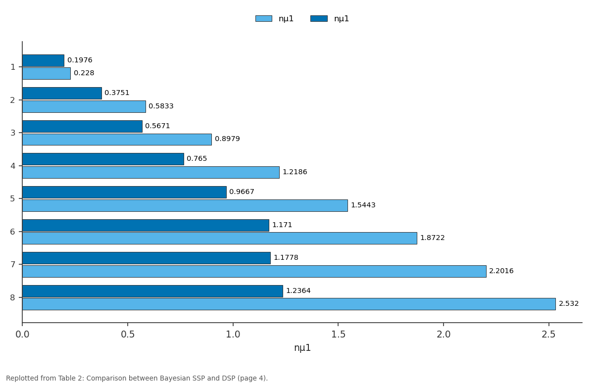
nµ1 and nµ1: 1 vs 2 vs 3 vs 4 vs 5
Replotted from Table 2 (page 4) of the original paper. Every bar is the paper's own table value.
View source evidence ↗Figures & tables
From the original paper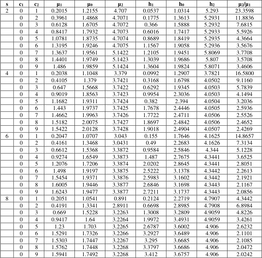 Table 1
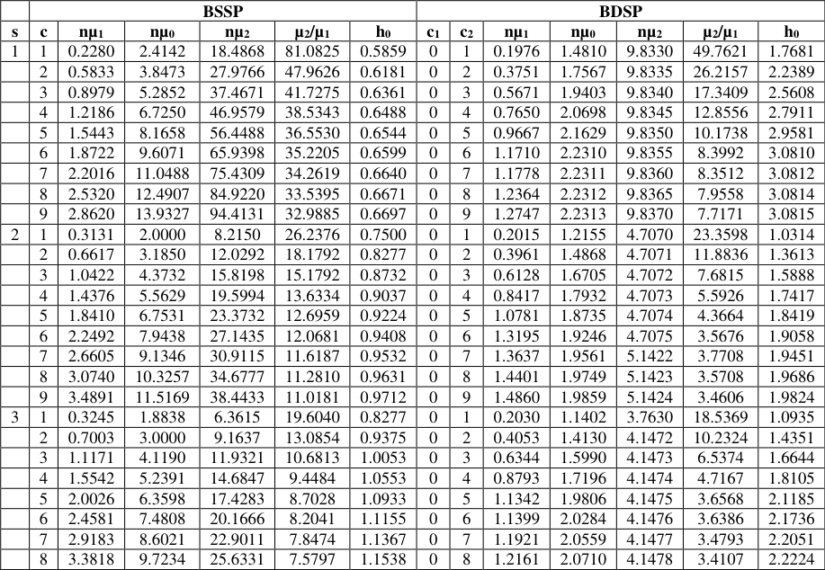 Table 2
Introduction
Since the beginning of various statistical concepts, methods and techniques are used to furnish lot by lot acceptance sampling plan. Inspection of the lot and final product is very necessary to ensure good quality. In fact the theory of sampling inspection pays more attention to improve the quality and reduce cost in terms of minimum sample size. In this scenario industrialists are able to bring innovative production with the help of Bayesian sampling plan, which is more effective than existing sampling plan, taking smaller inspection cost and efficiency over sample size. The basic assumption in all the sampling plans is that the lot or process fraction defective is constant, which specifies the production process is stable. However, in real-life situations, the lots formed from a process will have quality variations which are due to random fluctuations. These variations are classified as within-lot variation and the other is between-lot variation. When the second type of variation is more than the first type of variation, the fraction defective items in the lots will vary continuously. In such cases, the conventional sampling plans cannot be applied. It is very important to note that acceptance sampling plans based on Bayesian methodology can be used when the experimenter has prior knowledge on the process variation to make a decision about the disposition of the lot. The prior distribution describes the user belief to the sample, about the defectives from lot-tolot. A decision to accept or reject the lot based on posterior distribution which combines the user prior knowledge of lot-to-lot variations with sampling inspection results. Bayesian sampling plan has a clear picture on the consequences associated with the selection of particular prior distribution. Thus, the pitfalls in the selection of a prior distribution have been pointed out by Case and Keats (1982) [2] . Calvin (1984) [1] has presented clearly and concisely the meaning of 'how and when to perform Bayesian Acceptance Sampling'. These procedures are suited to the sampling of lots either process or assembly operations, that contain assignable causes. Such causes may be unknown and awaiting isolation, known but irremovable due to the state of limitations, or known but uneconomical to remove. Further, theoretically if any major shift requires reassessment of the sampling plan, the accurate sampling risks were to be maintained. A set of tables presented by Oliver and Springer (1972) [7] based on assumption of Beta prior distribution with specific posterior risk, to achieve minimum sample size which avoids the issue of estimating cost parameters. It is generally true that, Bayesian plan requires smaller sample size than conventional sampling plan with the same producer and consumer risk. Hamaker and Vanstrik (1955) [5] studied the efficiency of double sampling attributes using indifference quality level and presented expressions for p 0 and h 0 . Dodge and Romig (1959) [3] have presented tables for double sampling plan indexed by AOQL and LTPD. Suresh (1993) [13] has presented and constructed tables for the selection of double sampling plan indexed through (p 1 ,h 1 ) and (p 2 ,h 2 ) involving incentive and filter effects. Suresh and Saminathan (2010) [11] have studied designing of Repetitive deferred sampling plan indexed through relative slopes and compared with Repetitive group sampling plan. Latha (2002) [6] studied the Bayesian single sampling plan indexed with various quality levels and relative slopes at indifference quality levels. Suresh et al (2013) [10] have studied designing of Bayesian Repetitive Deferred Sampling Plan (BRDS) indexed through incoming and outgoing quality levels with their relative slopes on the OC curve. Balamurali et al (2012) [8] have developed Bayesian double sampling plan that uses two quality levels. This plan is better than single sampling plan in terms of minimum ASN and lesser ASN than existing sampling plans. Suresh and Usha (2016) [12] have studied Bayesian double sampling plan using minimum angle method which is better than Bayesian single sampling plan in terms of minimizing tangent θ and two risks. Based on the above, the present work is attempted for Bayesian double sampling plan indexed through relative slopes at specified quality levels and comparison made with Bayesian single sampling plan (BSSP) with their quality levels. The present work would be worthy and useful in the area of quality control towards minimum sample size and efficiency through inspection cost.
Bayesian Double Sampling Plan
In general settings, DSP plan is authentic for application of attribute sampling inspection. However, this plan will especially be useful for product characteristics towards cost or involving destructive testing. A double sampling plan can significantly reduce the costs for sampling inspection related to single-sampling plan for lots with very low or very high proportion defective because a decision can be made after taking the first sample. If the decision requires two samples, the sampling cost can be greater than those of single-sampling plan. accept the lot otherwise reject the lot. Gamma-Poisson distribution, which is also known as the negative binomial distribution, is one of the most widely used models in acceptance sampling plans. When the production process produces output in a continuous stream and observed number of defects (or nonconformities) in the sample drawn from this process is distributed as Poisson with parameter np, where n is the sample size and p is the average number of defects per unit (Hald, 1981) [4] . According to Schilling (1982) [9] , the Poisson distribution is an appropriate model for the number of nonconforming items in the sample when the ratio of sample size to the population size is less than 10%, is (n/N) n is large and p<0.10 is small such that np<5. Double Sampling Plan is specified with constants n 1 and n 2 . It is assumed that n 1 = n 2 =n. Under the conditions of applications of Poisson model, the probability of acceptance of the double sampling plan given by
Operating
Here s is specified from the prior information about the production process. The posterior distribution for nonconformities is reduced under gamma-Poisson distribution. When the production is unstable, the nonconforming item (d) and average number of defects p are independently distributed. According to Hald (1981), the nonconforming items (d) can be developed under the process average
In order to continue this, the probability of acceptance of the double sampling plan under gamma-Poisson model is given by (4)
Selection of Bayesian Double Sampling (BDSP)
A double sampling plan gives similar levels of consumer and producer risk but require less sampling in the long run than a single sampling plan which is given in conventional sampling plan. Bayesian double sampling plan also better than Bayesian single sampling plan, further comparison are given for BDSP and BSSP .
Designing of Bayesian Double Sampling Plan indexed through Relative Slopes
Designing procedures for quality levels namely, Acceptable Quality Level (AQL), Indifference Quality Level (IQL) and Limiting Quality Level (LQL) are considered with their corresponding relative slopes (denoted by h), to describe the degree of sharpness for the OC curve.
Selection of BDSP Relative slope at AQL, IQL and LQL Example 2
Selection of BDSP Relative slope at AQL, IQL and LQL Example 2
Comparative study on Single and Double Sampling Plan under Bayesian Methodology
Table 2 is shows that Bayesian single sampling plan and Bayesian double sampling plan for given various parametric values of 's' and relative slope at indifference quality levels.
| — | BSSP | — | — | — | — | — | BDSP | — | — | — | — | — | — |
|---|---|---|---|---|---|---|---|---|---|---|---|---|---|
| s | c | nµ1 | nµ0 | nµ2 | µ2/µ1 | h0 | c1 | c2 | nµ1 | nµ0 | nµ2 | µ2/µ1 | h0 |
| 1 | 1 | 0.2280 | 2.4142 | 18.4868 | 81.0825 | 0.5859 | 0 | 1 | 0.1976 | 1.4810 | 9.8330 | 49.7621 | 1.7681 |
| 2 | 0.5833 | 3.8473 | 27.9766 | 47.9626 | 0.6181 | 0 | 2 | 0.3751 | 1.7567 | 9.8335 | 26.2157 | 2.2389 | |
| 3 | 0.8979 | 5.2852 | 37.4671 | 41.7275 | 0.6361 | 0 | 3 | 0.5671 | 1.9403 | 9.8340 | 17.3409 | 2.5608 | |
| 4 | 1.2186 | 6.7250 | 46.9579 | 38.5343 | 0.6488 | 0 | 4 | 0.7650 | 2.0698 | 9.8345 | 12.8556 | 2.7911 | |
| 5 | 1.5443 | 8.1658 | 56.4488 | 36.5530 | 0.6544 | 0 | 5 | 0.9667 | 2.1629 | 9.8350 | 10.1738 | 2.9581 | |
| 6 | 1.8722 | 9.6071 | 65.9398 | 35.2205 | 0.6599 | 0 | 6 | 1.1710 | 2.2310 | 9.8355 | 8.3992 | 3.0810 | |
| 7 | 2.2016 | 11.0488 | 75.4309 | 34.2619 | 0.6640 | 0 | 7 | 1.1778 | 2.2311 | 9.8360 | 8.3512 | 3.0812 | |
| 8 | 2.5320 | 12.4907 | 84.9220 | 33.5395 | 0.6671 | 0 | 8 | 1.2364 | 2.2312 | 9.8365 | 7.9558 | 3.0814 | |
| 9 | 2.8620 | 13.9327 | 94.4131 | 32.9885 | 0.6697 | 0 | 9 | 1.2747 | 2.2313 | 9.8370 | 7.7171 | 3.0815 | |
| 2 | 1 | 0.3131 | 2.0000 | 8.2150 | 26.2376 | 0.7500 | 0 | 1 | 0.2015 | 1.2155 | 4.7070 | 23.3598 | 1.0314 |
| 2 | 0.6617 | 3.1850 | 12.0292 | 18.1792 | 0.8277 | 0 | 2 | 0.3961 | 1.4868 | 4.7071 | 11.8836 | 1.3613 | |
| 3 | 1.0422 | 4.3732 | 15.8198 | 15.1792 | 0.8732 | 0 | 3 | 0.6128 | 1.6705 | 4.7072 | 7.6815 | 1.5888 | |
| 4 | 1.4376 | 5.5629 | 19.5994 | 13.6334 | 0.9037 | 0 | 4 | 0.8417 | 1.7932 | 4.7073 | 5.5926 | 1.7417 | |
| 5 | 1.8410 | 6.7531 | 23.3732 | 12.6959 | 0.9224 | 0 | 5 | 1.0781 | 1.8735 | 4.7074 | 4.3664 | 1.8419 | |
| 6 | 2.2492 | 7.9438 | 27.1435 | 12.0681 | 0.9408 | 0 | 6 | 1.3195 | 1.9246 | 4.7075 | 3.5676 | 1.9058 | |
| 7 | 2.6605 | 9.1346 | 30.9115 | 11.6187 | 0.9532 | 0 | 7 | 1.3637 | 1.9561 | 5.1422 | 3.7708 | 1.9451 | |
| 8 | 3.0740 | 10.3257 | 34.6777 | 11.2810 | 0.9631 | 0 | 8 | 1.4401 | 1.9749 | 5.1423 | 3.5708 | 1.9686 | |
| 9 | 3.4891 | 11.5169 | 38.4433 | 11.0181 | 0.9712 | 0 | 9 | 1.4860 | 1.9859 | 5.1424 | 3.4606 | 1.9824 | |
| 3 | 1 | 0.3245 | 1.8838 | 6.3615 | 19.6040 | 0.8277 | 0 | 1 | 0.2030 | 1.1402 | 3.7630 | 18.5369 | 1.0935 |
| 2 | 0.7003 | 3.0000 | 9.1637 | 13.0854 | 0.9375 | 0 | 2 | 0.4053 | 1.4130 | 4.1472 | 10.2324 | 1.4351 | |
| 3 | 1.1171 | 4.1190 | 11.9321 | 10.6813 | 1.0053 | 0 | 3 | 0.6344 | 1.5990 | 4.1473 | 6.5374 | 1.6644 | |
| 4 | 1.5542 | 5.2391 | 14.6847 | 9.4484 | 1.0553 | 0 | 4 | 0.8793 | 1.7196 | 4.1474 | 4.7167 | 1.8105 | |
| 5 | 2.0026 | 6.3598 | 17.4283 | 8.7028 | 1.0933 | 0 | 5 | 1.1342 | 1.9806 | 4.1475 | 3.6568 | 2.1185 | |
| 6 | 2.4581 | 7.4808 | 20.1666 | 8.2041 | 1.1155 | 0 | 6 | 1.1399 | 2.0284 | 4.1476 | 3.6386 | 2.1736 | |
| 7 | 2.9183 | 8.6021 | 22.9011 | 7.8474 | 1.1367 | 0 | 7 | 1.1921 | 2.0559 | 4.1477 | 3.4793 | 2.2051 | |
| 8 | 3.3818 | 9.7234 | 25.6331 | 7.5797 | 1.1538 | 0 | 8 | 1.2161 | 2.0710 | 4.1478 | 3.4107 | 2.2224 |
Table text extracted from the original PDF; superscript letters are shown inline. The original table image is below.
View original table image
Selection through AQL and LQL
It is observed that the both plan are quite similar in nature of sampling procedures. If their OC curves are identical and two plans would be considered as matched. The proposed plan is better than Bayesian single sampling plan in terms of minimizing the sample size.
Construction of Tables
The relative slope is, ,, h h h are obtained in Table 1.
| s | c1 | c2 | µ1 | µ0 | µ2 | h1 | h0 | h2 | µ2/µ1 |
|---|---|---|---|---|---|---|---|---|---|
| 2 | 0 | 1 | 0.2015 | 1.2155 | 4.707 | 0.0537 | 1.0314 | 5.293 | 23.3598 |
| 0 | 2 | 0.3961 | 1.4868 | 4.7071 | 0.1775 | 1.3613 | 5.2931 | 11.8836 | |
| 0 | 3 | 0.6128 | 1.6705 | 4.7072 | 0.366 | 1.5888 | 5.2932 | 7.6815 | |
| 0 | 4 | 0.8417 | 1.7932 | 4.7073 | 0.6016 | 1.7417 | 5.2933 | 5.5926 | |
| 0 | 5 | 1.0781 | 1.8735 | 4.7074 | 0.8689 | 1.8419 | 5.2935 | 4.3664 | |
| 0 | 6 | 1.3195 | 1.9246 | 4.7075 | 1.1567 | 1.9058 | 5.2936 | 3.5676 | |
| 0 | 7 | 1.3637 | 1.9561 | 5.1422 | 1.2105 | 1.9451 | 5.8069 | 3.7708 | |
| 0 | 8 | 1.4401 | 1.9749 | 5.1423 | 1.3039 | 1.9686 | 5.807 | 3.5708 | |
| 0 | 9 | 1.486 | 1.9859 | 5.1424 | 1.3604 | 1.9824 | 5.8071 | 3.4606 | |
| 4 | 0 | 1 | 0.2038 | 1.1048 | 3.379 | 0.0992 | 1.2907 | 3.7821 | 16.5800 |
| 0 | 2 | 0.4105 | 1.379 | 3.7421 | 0.3168 | 1.6798 | 4.0502 | 9.1160 | |
| 0 | 3 | 0.647 | 1.5668 | 3.7422 | 0.6292 | 1.9345 | 4.0503 | 5.7839 | |
| 0 | 4 | 0.9019 | 1.8563 | 3.7423 | 0.9954 | 2.3036 | 4.0503 | 4.1494 | |
| 0 | 5 | 1.1682 | 1.9311 | 3.7424 | 0.382 | 2.394 | 4.0504 | 3.2036 | |
| 0 | 6 | 1.443 | 1.9737 | 3.7425 | 1.7678 | 2.4446 | 4.0505 | 2.5936 | |
| 0 | 7 | 1.4662 | 1.9963 | 3.7426 | 1.7722 | 2.4711 | 4.0506 | 2.5526 | |
| 0 | 8 | 1.5182 | 2.0075 | 3.7427 | 1.8697 | 2.4842 | 4.0506 | 2.4652 | |
| 0 | 9 | 1.5422 | 2.0128 | 3.7428 | 1.9018 | 2.4904 | 4.0507 | 2.4269 | |
| 6 | 0 | 1 | 0.2047 | 1.0707 | 3.043 | 0.155 | 1.7646 | 4.1625 | 14.8657 |
| 0 | 2 | 0.4161 | 1.3468 | 3.0431 | 0.49 | 2.2683 | 4.1626 | 7.3134 | |
| 0 | 3 | 0.6612 | 1.5368 | 3.3872 | 0.9584 | 2.5846 | 4.344 | 5.1228 | |
| 0 | 4 | 0.9274 | 1.6549 | 3.3873 | 1.487 | 2.7675 | 4.3441 | 3.6525 | |
| 0 | 5 | 1.2076 | 1.7206 | 3.3874 | 2.0202 | 2.8645 | 4.3441 | 2.8051 | |
| 0 | 6 | 1.498 | 1.9197 | 3.3875 | 2.5222 | 3.1378 | 4.3442 | 2.2613 | |
| 0 | 7 | 1.5454 | 1.9371 | 3.3876 | 2.5983 | 3.1602 | 4.3442 | 2.1921 | |
| 0 | 8 | 1.6005 | 1.9446 | 3.3877 | 2.6846 | 3.1698 | 4.3443 | 2.1167 | |
| 0 | 9 | 1.6243 | 1.9477 | 3.3877 | 2.7211 | 3.1737 | 4.3443 | 2.0856 | |
| 8 | 0 | 1 | 0.2051 | 1.0541 | 0.891 | 0.2124 | 2.2719 | 4.7907 | 4.3442 |
| 0 | 2 | 0.4191 | 1.3341 | 2.8911 | 0.6698 | 2.8985 | 4.7908 | 6.8984 | |
| 0 | 3 | 0.669 | 1.5228 | 3.2263 | 1.3008 | 3.2809 | 4.9059 | 4.8226 | |
| 0 | 4 | 0.9417 | 1.64 | 3.2264 | 1.9972 | 3.4931 | 4.9059 | 3.4261 | |
| 0 | 5 | 1.23 | 1.703 | 3.2265 | 2.6787 | 3.6002 | 4.906 | 2.6232 | |
| 0 | 6 | 1.5291 | 1.7326 | 3.2266 | 3.2927 | 3.6489 | 4.906 | 2.1101 | |
| 0 | 7 | 1.5303 | 1.7447 | 3.2267 | 3.295 | 3.6685 | 4.906 | 2.1085 | |
| 0 | 8 | 1.5762 | 1.7448 | 3.2268 | 3.3797 | 3.6686 | 4.906 | 2.0472 | |
| 0 | 9 | 1.5941 | 1.7492 | 3.2268 | 3.412 | 3.6757 | 4.906 | 2.0242 |
Table text extracted from the original PDF; superscript letters are shown inline. The original table image is below.
View original table image
Conclusions
The present work is mainly related to the construction and selection of BDSP through various quality levels and relative slopes. In order to build confidence among producer and consumer towards minimize the sample size and risks. The effectiveness of this procedure is evaluated by comparing its results with those of obtained from optimal Bayesian acceptance sampling plan. Tables provided here with tailormade, handy ready-made can be used in the industrial shopfloor condition. This result would be assistance in the field of quality control to develop new plans and procedures for engineer and plan designers.
Acknowledgement
AcknowledgementsThe second author is thankful to Department of Science and Technology, New Delhi, towards providing DST-Inspire fellowship for carrying out this research work. The first author is thankful to University Grants Commissions, New Delhi, for providing UGC-OTG for financial support.
References
13 in the original paper- Calvin TW. How and when to perform Bayesian Acceptance Sampling, American Society for Quality Control, Vol.7, Milwaukee, Wisconsin, 1984.
- Case KE, Keats JB. On the selection of a Prior Distribution in Bayesian Acceptance Sampling. Journal of Quality Technology. 1982; 14(1):10-18.
- Dodge HF, Romig HG. Sampling Inspection TablesSingle and Double Sampling, 2 nd Edition, John Wiley and Sons, New York, 1959.
- Hald A. Statistical Theory of Sampling Inspection by Attributes, Academic Press, New York, 1981.
- Hamaker HC, Van Strik R. The Efficiency of Double Sampling for Attributes. Journal of the American Statistical Association. 1955; 50(271):830-849.
- Latha M. Certain Studies Relating to Bayesian Acceptance Sampling Plan, Ph.D Thesis, Department of Statistics, Bharathiar University, Tamilnadu, 2002.
- Oliver LR, Springer MD. A General set of Bayesian Attribute Acceptance Plans, American Institute of industrial Engineers, Norcross, G.A., 1972.
- Saminathan Balamurali, Muhammad Aslam, Chi-Hyuck Jun. Bayesian Double Sampling Plan under the GammaPoisson Distribution. Research Journal of Applied Sciences, Engineering and Technology. 2012; 4(8):949956.
- Schiling EG. Acceptance Sampling in Quality Control, Marcel Dekker, New York, 1982.
- Suresh KK, Umamaheswari S, Pradeepa Veerakumari K. Bayesian Repetitive Deferred Sampling Plan Indexed Through Relative Slopes. Mathematical Journal of Interdisciplinary Sciences. 2013; 1(2): 41-54.
- Suresh KK, Saminathan R. Construction and Selection of Repetitive Deferred Sampling plan through Acceptable and Limiting Quality Levels. International Journal of Pure and Applied Mathematics. 2010; 65(3):257-264.
- Suresh KK, Usha K. Construction of Bayesian double sampling plan using minimum angle method. Journal of Statistics and Management System. 2016; 19(3):473-489.
- Suresh KK. A study on Acceptance Sampling using Acceptable and Limiting Quality levels, Ph.D Thesis, Bharathiar University, Tamilnadu, 1993.