
Research article · 2018 · Full text
International Journal of Statistics and Applied MathematicsA study on analytical solution for acoustic waves propagation in fluids
Volume 3(1) · Pages 54–59
Research areasUnderwater Acoustics ResearchFlow Measurement and AnalysisUltrasonics and Acoustic Wave Propagation
Abstract
Author-writtenIn this paper, The approach is based on a analytical solution to the homogeneous wave equation for fluid medium. Analytical solution found for the acoustic waves propagation in fluid medium using normal mode analysis and discuss the computational results.
Summary
Source-checkedPlain-language reading of the full paper, prepared with AI and checked against the text. Each point links to the authors' own words.
Why it matters
- Physical acoustic wave modeling is a valuable tool for applications in therapeutic and diagnostic ultrasound. View evidence ↗
- While numerical methods are used for sound field simulation, they can be computationally expensive and memory-intensive when modeling waves over large distances. View evidence ↗
- Normal mode analysis is an alternative that provides exact solutions without requiring assumed restrictions on velocity and pressure distributions. View evidence ↗
The question
- The study aims to use normal mode analysis to find an analytical solution for the linear acoustic wave equation. View evidence ↗
What they did
- The research focuses on the propagation of acoustic pressure waves in a medium with two-dimensional spatially variable acoustic properties. View evidence ↗
- The analysis is based on Euler's equation and the equation of continuity for sound waves propagating in water within a two-dimensional space. View evidence ↗
What they found
- The peak wave amplitude decreases as the distance from the source increases. View evidence ↗
- Higher wave frequencies result in increased attenuation at any specific location. View evidence ↗
- At a fixed distance of x = 2 cm, the magnitude of the peak pressure shows very little change relative to the frequency. View evidence ↗
What it means
- The authors concluded that the developed normal mode analysis accurately models the pressure acoustic wave equation and is characterized by speed and simplicity in design and implementation. View evidence ↗
- The authors suggest that future work could involve using the model to incorporate non-linear propagation effects. View evidence ↗
Visual summary
1 visualsIllustrations explain the paper; they do not show study data.
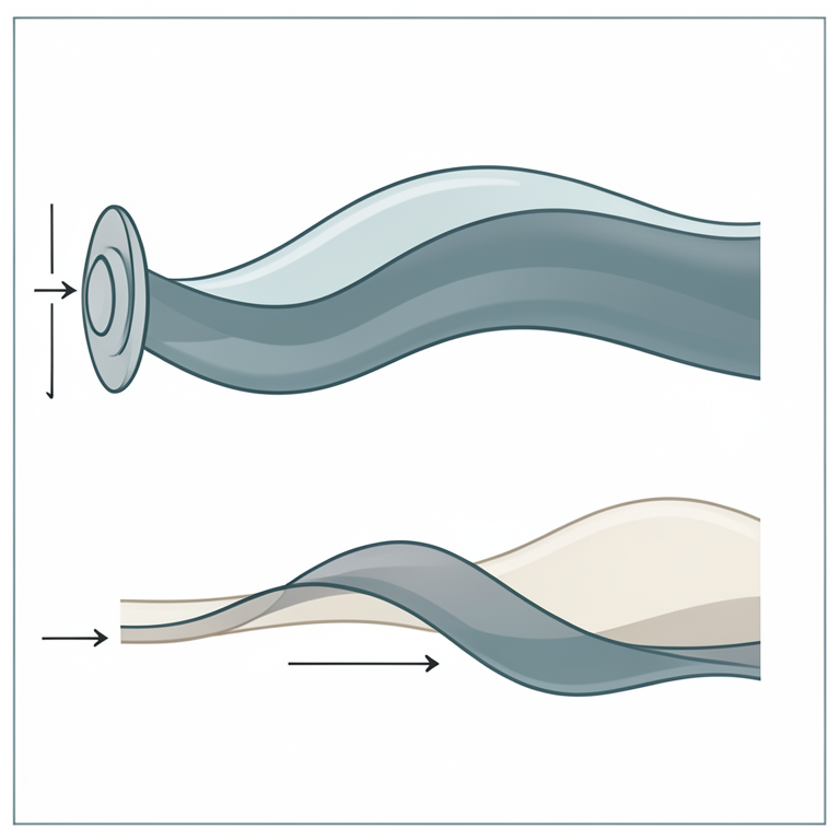
Acoustic Wave Attenuation
AI-generated conceptual illustration (acoustic waves in a fluid medium). It explains the idea and does not show study data.
View source evidence ↗Figures & tables
From the original paper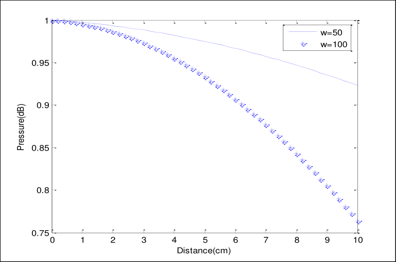 Figure 1
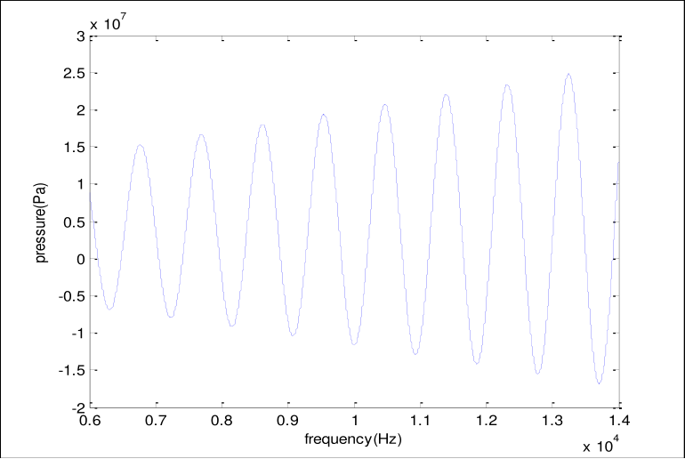 Figure 2
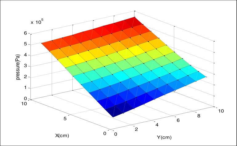 Figure 3
Introduction
In recent years, physical acoustic wave modeling has become a successful tool in diagnostic and therapeutic ultrasound application. There are several wave equations available for describing acoustic wave propagation. Numerical methods can be used as a tool for sound field simulation. Discrete-time simulation algorithms for wave propagation can be derived by numerically solving an acoustic wave equation in terms of the variables for sound pressure and particle velocity.
Initial conditions for time derivatives and boundary conditions for space derivatives are necessary to provide a complete set of solutions of the wave equation. These equations are most commonly solved by propagation in time. However, when propagating over large distances, such methods are expensive in terms of memory and computational costs. The normal mode analysis method gives exact solutions without any assumed restrictions on pressure and velocity components distributions.
It is applied to wide range of problems in different branches. It can be applied to boundary-layer problems, which are described by the linearized Navier-stokes equations in electrohydrodynamic. In this paper, the normal mode analysis can be employed to solve linear acoustic wave equation analytically. The technique focuses on description of a linear model and discuses the conditions under which using this technique.
The propagation of acoustic pressure wave by the normal mode analysis in a medium with two-dimensional spatially variable acoustic properties has been explained. 2. Acoustic Wave Equation Consider sound waves propagating in the water. Instead of the wave equation, we base our work on the basic Euler’s equation and the equation of continuity. For simplicity, the
Discussion
is confined to a two dimensional space. In a 2-D Cartesian coordinate system, the sound pressure p and the particle velocity v satisfy the following linear equations: t y x p ) 1 . 2 ...( ) , , ( 1 ) , , ( . 2 c t y x v t t y x p t y x v x ) 2 . 2 ...( ) , , ( ) , , ( x t t y x v t y x p y ) 3 . 2 ....( ) , , ( ) , , ( y t Maths 2018; 3(1): 54-59 M Muthukani Assistant Professor, KG College of Arts and Science, Coimbatore, Tamil Nadu, India Correspondence M Muthukani Assistant Professor, KG College of Arts and Science, Coimbatore, Tamil Nadu, India is the particle velocity, ) , , ( t y x p is the pressure and is the density of the where ) , , ( ˆ ) , , ( ˆ ) , , ( t y x v y t y x v x t y x v y x fluid with wave number i c k where 1 i , is angular frequency, c and are the speed of sound and attenuation in homogenious medium, respectively. Normal Mode Analysis The solution of considered physical variable can be decomposed in terms of normal modes as the following form ) ( * * * ky t i ) 4 . 2 ...( ) ]( , , [ ) , , ]( , , [ y x y x e x p v v t y x p v v Where * p are the amplitude of the functions x x v v , and p respectively. * * , y x v v and Equation (2.1) becomes t y x p ) , , ( 1 ) , , ( . 2 t c t y x v t y x p ) , , ( 1 )) , , ( ˆ ) , , ( ˆ )( ˆ ˆ ( y x 2 t c t y x v y t y x v x y y x x t y x v t y x v t y x p y x ) , , ( 1 ) ) , , ( ) , , ( ( 2 x t c y Apply equation (2.4) in above equation ) ( * ) ( * ky t i ky t i ) ( * e x v e x v e x p y ky t i x ) ( 1 ) ) ( ) ( ( 2 x y t c ) ( * ) ( * ky t i ky t i ky t i ) ( * . ) ( 1 ) . ) ( ) ( ( i e x p ik e x v e x Dv x y 2 c ky t i * * ) ( ) ( * ky t i e x p i kv i Dv e ) ( ) ( y x 2 c * * * p i kv i Dv ) 5 . 2 ...( y x 2 c Applying (2.4) in Equation (2.2) * x p ) ( ) ( ) ( * ) ( ky t i x ky t i x v e x e t ) ( * ) ( * ky t i ky t i i e v e Dp . x * * v i Dp ) 6 . 2 ...( . x Applying (2.4) in equation (2.3) * x p ) ( ) ( ) ( * ky t i y ky t i ) ( x v e y e t ) ( * ) ( * ky t i ky t i i e v ik e p . . y * * v kp ) 7 . 2 ...( . y Where x D Equation (2.5) – (2.7) form a coupled system. * * Eliminating x v and y v values in equation (2.5) * * ) 8 . 2 ...( 1 x Dp i v * * p k v ) 9 . 2 ...( y * * Substitute x v and x v values in equation (2.5) * * * ) ( ) 1 ( 2 i p k k i Dp i D p c 2 * 2 * 2 * i p ik p iD 2 p c 2 * 2 * 2 * 0 2 p c p k p D 2 2 * 2 * 0 2 p c k p D * 2 * 2 p m p D ) 10 . 2 ...( 0 2 2 2 2 c k m Where, The solution of equation (2.10) has the form 2 ) 11 . 2 ...( ) ( i p x p * * i 1 x r Where i i i e k G p ) , ( * , and r i are the roots of the characteristic equation. m r ) 12 . 2 ...( 0 2 2 i m r i T he solution of equation (2.10) is given by * mx mx e k G e k G x p ) 13 . 2 ...( ) , ( ) , ( ) ( 2 1 Substitute * p values in equation (2.8) * mx mx ) ) , ( ) , ( ( 1 x 2 1 e k G e k G D i v mx mx ) ) , ( ) , ( ( 1 2 1 e k mG e k mG i * mx mx m v ) 14 . 2 ...( ) , ( ) , ( x 2 1 m e k G i e k G i * ' mx mx ' e k G e k G v ) 15 . 2 ...( ) , ( ) , ( x 1 2 ' ' m k G Where ) 16 . 2 ...( ) , ( ) , ( , ) , ( ) , ( 2 2 1 1 k G i m k G k G i Substitute * p values in equation (2.9) * mx mx e k G e k G k v ) ) , ( ) , ( ( y 2 1 * mx mx e k G k e k G k v ) 17 . 2 ...( ) , ( ) , ( y 2 1 * '' '' mx mx e k G e k G v ) 18 . 2 ...( ) , ( ) , ( y 1 2 '' '' 2 1 Where ) 19 . 2 ...( ) , ( ) , ( , ) , ( ) , ( 2 1 k G k k G k G k k G Boundary Condition On the surface at x=0 * * t y p p t y F v x ) 20 . 2 ...( ) , ( , ) , ( 0 Substituting from (2.4) into (2.20) * * * * , p p F v x 0 0 at x=0 equation (2.13) becomes ) 21 . 2 ...( 2 1 * 0 G G p Equation (2.14) becomes * m F ) ( 0 2 1 G G i i * ) 22 . 2 ...( 0 2 1 G G F m By adding equation (2.21) and (2.22) we obtain i p G 1 * 0 * 0 1 F m ) 23 . 2 ...( ) ( 2 By subtracting equation (2.21) and (2.22) we obtain 1 * * i p G 0 0 2 F m ) 24 . 2 ...( ) ( 2 By substituting from equation (2.23) and (2.24) into the equation (2.13),(2.14) and (2.17) ) ( * ky t i e x p t y x p ) ( ) , , ( ky t i mx mx e e k G e k G t y x p ) 25 . 2 ....( ) ) , ( ) , ( ( ) , , ( ) ( 2 1 ) ( * e v t y x v ) , , ( ky t i x x m t y x v ) 26 . 2 ....( ) ) , ( ) , ( ( ) , , ( ky t i mx mx x ) ( 2 1 e e k G e k G i ) ( * e v t y x v ) , , ( ky t i y y e e k G e k G k t y x v ) 27 . 2 ....( ) ) , ( ) , ( ( ) , , ( ky t i mx mx y ) ( 2 1 3. Computational Results To study the wave propagation phenomenon in viscous medium and under different frequencies, we can apply the theoretical acoustic viscous wave Equation (2.25).
Using water as the medium, the parameters are given as following: 3 998 m Kg * and s m c 1481 . Let the wave peak amplitude be Pa p 1 0 at the source (x=0), we simulate the 0 and s m F 1 * pressure wave peak amplitude, in Equation (2.25), the distance from the source at various frequencies. The results are shown in Figure 1 (in dB and linear scale). As expected, the peak wave amplitude becomes smaller as we move further from the source.
We can also notice that as the wave frequency goes higher, more attenuation can be observed at any given location. The peak pressure as function of frequency shown in Figure 2 for fixed distance at x = 2 cm. It is clear from this figure that the magnitude of peak of pressure little changes with the frequency. Let us consider a 2-D simulation in which the pressure varies in the x and y directions.
Figure 3 shows the 2-D pressure computational as function in the plane x-y. From this figure, it can be seen that the pressure amplitude becomes smaller when moving in the x-y plane further from the source. Pressure amplitude (dB) as function of the distance from the origin 1 w=50 w=100 0.95 0.9 Pressure(dB) 0.85 0.8 0 1 2 3 4 5 6 7 8 9 10 0.75 Distance(cm) Fig 1 The pressure amplitude as function of frequency at distance 2 cm from the source 7 3 x 10 2.5 2 1.5 1 0.5 pressure(Pa) 0 -0.5 -1 -1.5 -2 0.6 0.7 0.8 0.9 1 1.1 1.2 1.3 1.4 4 frequency(Hz) x 10 Fig 2 The pressure amplitude as function of plane x-y direction 5 x 10 6 5 4 3 2 pressure(Pa) 1 0 10 10 8 5 6 4 2 0 0 Y(cm) X(cm) Fig 3
Conclusion
A normal mode analysis which accurately the pressure acoustic wave equation, has been developed. This technique has a number of attractive features, foremost of which is the speed and simplicity with which it can be designed and implemented. The model could be used in the future to incorporate non-linear propagation effects.
References
6 in the original paper- Bill Drafts. Acoustic Wave Technology Sensors, Microsensor Systems Inc, 2000.
- Jeanne M Hossenlopp. Applications of Acoustic Wave Devices for Sensing in Liquid Environments, Marquette University, 2006.
- Lawerence E Kinsler, Austin R Frey. Fundamentals of Acoustics, Second edition, John wiley and sons INC, New York 1962.
- Mohamed I. A. Othman, Mohamed Galal Sayed Ali, Roushdi Mohamed Farouk., Analytical Solution For Acoustic Waves Propagation In Fluids, World Journal of Mechanics, 2011.
- Nirmala J. Structure of Liquid and Comparison of Adhesive Force with Cohesion Force, International Journal of Engineering, Science and Mathematics, 2017
- Rienstra SW, Hirsch berg A. An Introduction to Acoustics, Eindhoven University of Technology, Eindhoven, 2009.