
Research article · 2018 · Full text
International Journal of Statistics and Applied MathematicsChange point method with Rayleigh distribution
Volume 3(2) · Pages 614–620
Research areasTechnology and Data Analysis
Abstract
Author-writtenThis paper intends to assess the performance between CUSUM and change point model of Rayleigh distribution by considering ARLs respectively. Finally we conclude that the performance of change point model is superior to CUSUM chart in the context of Rayleigh distribution.
Summary
Source-checkedPlain-language reading of the full paper, prepared with AI and checked against the text. Each point links to the authors' own words.
Why it matters
- Statistical Process Control (SPC) is used to identify and diagnose when a process has deviated from its state of statistical control. View evidence ↗
- While Shewhart control charts are useful for isolated causes, they are less effective at detecting small, sustained changes, for which CUSUM and EWMA charts are typically used. View evidence ↗
- The Change Point formulation is a less common method for detecting sustained changes, particularly when process averages do not follow a Normal distribution. View evidence ↗
The question
- The study aims to compare the performance of the CUSUM chart and the change point model specifically for the Rayleigh distribution using Average Run Lengths (ARLs). View evidence ↗
What they did
- The research focuses on a scenario where all process parameters are unknown under varying distributions. View evidence ↗
- Control limits were determined through the simulation of 10 million sequences, each with a length of 200, using the Rayleigh distribution. View evidence ↗
- The simulation evaluated control limits for hazard rates (α) ranging from 0.05 to 0.001, which correspond to in-control ARLs from 20 to 1000, for sample sizes (n) between 3 and 200. View evidence ↗
- The primary simulation assumed that the first 9 readings were not tested, with formal change point testing beginning at the 10th observation. View evidence ↗
- To assess performance, shifts of size δ (ranging from 0 to 3) were introduced at various time points τ (10, 25, 50, 100, and 250). View evidence ↗
What they found
- The Average Run Length (ARL) tends to decrease when either the hazard rate (α) or the shift size (δ) is larger. View evidence ↗
- The response time (ARL) is influenced by the amount of data gathered before a shift occurs, with more history leading to a faster response. View evidence ↗
- The change point model outperformed the CUSUM chart with k=0.25 for small shifts and the CUSUM chart with k=0.5 for medium shifts. View evidence ↗
- For the Rayleigh distribution, the change point model was found to be the strongest diagnostic for detecting shifts in the process average compared to the CUSUM chart. View evidence ↗
What it means
- The authors conclude that the change point model is superior to the CUSUM chart when applied to the Rayleigh distribution. View evidence ↗
- The authors suggest that future research should investigate the behavior and performance of the change point model compared to the CUSUM chart across other non-normal distributions. View evidence ↗
Visual summary
1 visualsIllustrations explain the paper; they do not show study data.
Model Comparison Concept
AI-generated conceptual illustration (A digital signal waveform representing a Rayleigh distribution). It explains the idea and does not show study data.
View source evidence ↗Figures & tables
From the original paper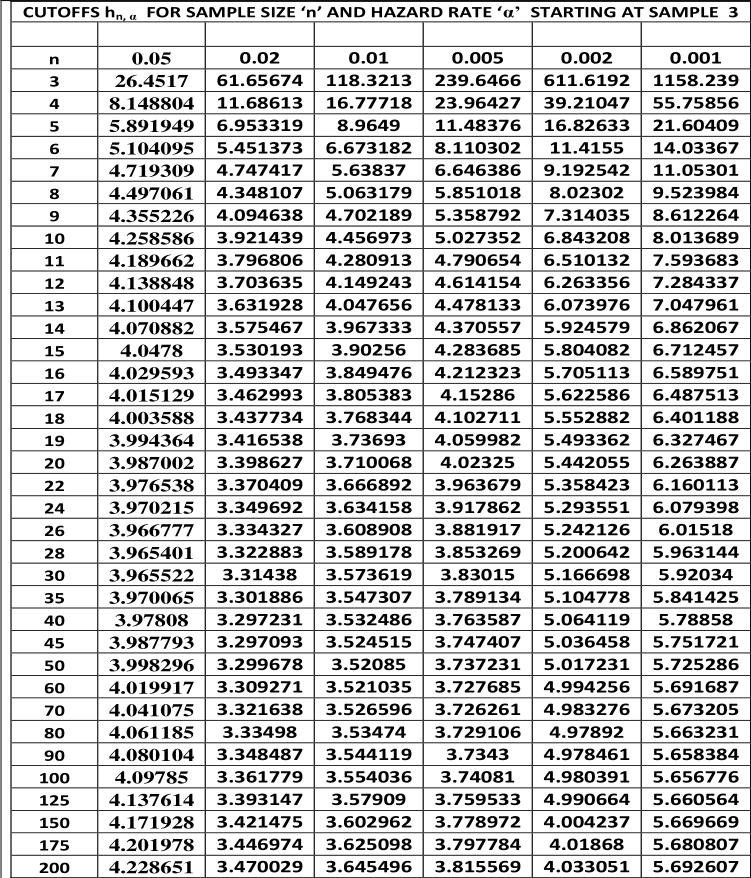 Table 3
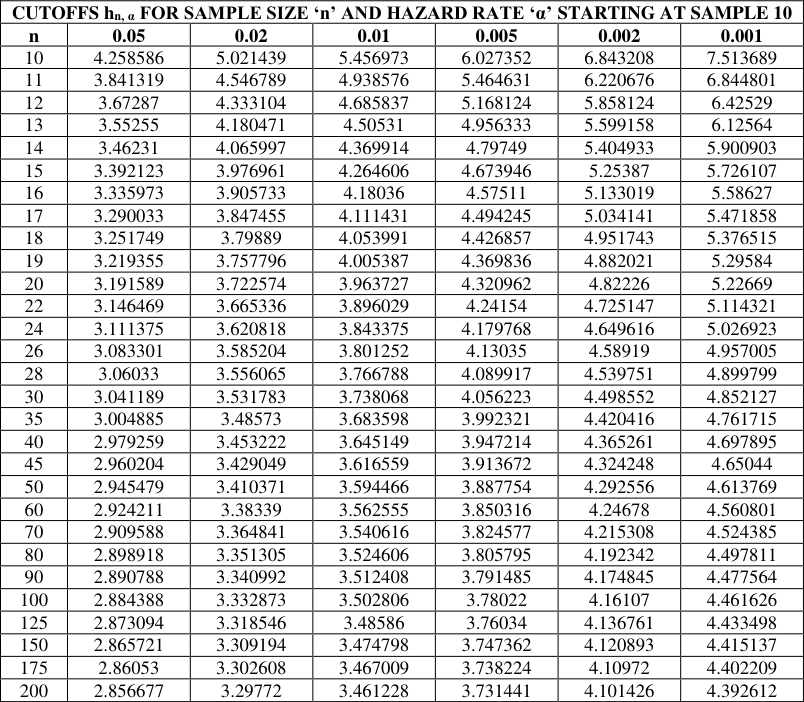 Table 3
 Table 4
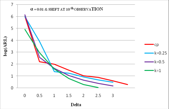 Figure 4
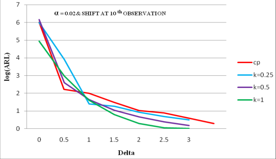 Figure 4
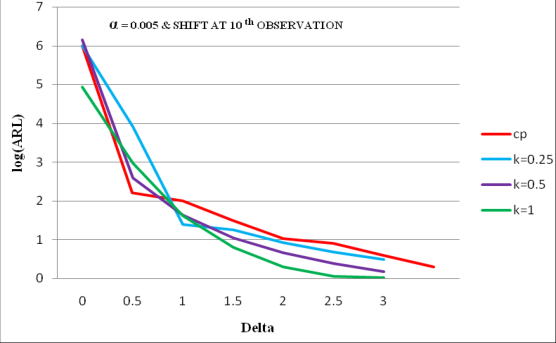 Figure 4
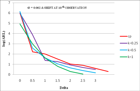 Figure 4
Introduction
The Statistical Process Control (SPC) aims to detect and diagnose situations where the process is gone out of statistical control. This type of problem involves two aspects namely process and statistical aspects. To have detailed outline of some of its statistical modeling aspects see Crowder et al. (1987) [1] . In fact the status of Statistical Quality Control may be described as one in which the process readings appear to follow a common statistical model. One model is that the process is in SQC, the successive process readings Xi's are independent and sampled from the same distribution. When the process goes out of control, it may behave in different ways. In general we can have two types of causes, those that affect single process readings and then disappear, and the second type of causes or sustainable causes. These causes will continue until they are identified and eliminated. In statistical terminology the isolated causes analogous to an out layer. The Shewart with an R or s-chart is an excellent tool for detecting these special causes, namely isolated or sustainable causes. However Shewart control char is less effective for detecting small changes in the process. Standard tools for detecting sustain changes are the CUSUM and EWMA chart. This paper focuses on another, less familiar; method aimed at detecting sustained changes is the Change Point formulation when the process averages follow non-Normal distribution.
Change point method
At first let us discuss Change Point Method when the process readings modeled by two Normal Distributions,
Here the number of observations 'n' is fixed in any traditional statistical settings, but this 'n' may increase unlimitedly in phase-II Statistical Process Control settings. Here both settings i.e. Phase-I and Phase-II will be discussed, with context indicating which of the two applies. In the case of in control distribution is N (μ1, σ1 2 ), the readings follows this distribution up to an epoch τ, the change point, at which point they shift to another Normal distribution different in mean i.e. μ1=μ2, in variability σ1 = σ2 or in both mean and variance. In change point method process readings leads to two statistical tasks namely testing task and estimating task. The testing task is to conform whether there has indeed being a change. If the change is there then the task of estimating τ, the time at which shift occurred. Sometimes we may have to estimate some or all of the parameters μ1, μ2, σ1 and σ2. In all discussions [see Hawkins, 2003] we work on change point has focused on shifts in mean only. i.e. μ1 ≠ μ2 but σ1 = σ2 = σ, throughout this paper this type of frame work is used here. From this change point method we have three scenarios based on the amount of process knowledge viz. All parameters μ1, μ2, σ1 and σ2 are known exactly priory. In control parameters μ and σ are known but μ2 is unknown. All parameters μ1, μ2, σ1 and σ2 are unknown. Throughout our discussions we concentrate on the third scenario namely all parameters are unknown under varying distributions.
Implementation of change point method
The formulae below mentioned indicate that the values are computationally burdensome. For the implementation of the method, construct two arrays of values of
( There is no need to store the running mean = , but it will be calculated 'on the fly'. The observation of the two new table entries can be calculated from the numerically stable recursions, when a new observation is added
The two sample statistic are calculated for every possible split point 1≤ j≤ n after finding (The customary variance estimator), using the value j leading to the maximum. The estimators are somewhat biased even though the maximum likelihood estimator are calculated by Hinkley (1970) [3] .
The maximizing j is that which maximizes jn E , so the searching step need only to evaluate Willsky and Jones (1976) [6] discussed the 'window' approach which is different from above method, in that observations more than w time periods into the past are not lost, since they are summarized in the window's leftmost S and W entry. The lost is the ability to split at these old instants. Appropriate values for the table size W may be in the 500 to 2000 range. It is very large as no interesting structure is lost, but small enough to compute for each new reading to less than 20000 operations.
Changepoint method with rayleigh distribution when the parameters are not know
Consider the model with none of the parameters known; we can test the presence of change point with another general Likelihood ration test. This test is a two sample t-test between before shift and after shift of the sequence, maximised across all possible change points; Worsely (1979) [7] . For a given change point 'j' where 1≤ j ≤ n-1, let
Be the mean of the (n-j) observations after shift. The residual sum of squares i.e. Vjn is given by
Here we assume that there is a single change point approach at epoch 'j', For a stable process, Tjn follows at t-distribution with n-2 degrees of freedom. An out of control signal is obtain as soon as
Exceeds some critical value, hn. Hawkins et al. (2003) [2] showed that, for any type I error, hn can be computed by using the Bonferroni inequality. They mentioned that the latter is conservative when a process measurement (n) is large. At same time, they provide empirical control limits, hn, α for different type I error, α, and various number of process observations. Also, for large n values (n≥1), they proposed the following approximation formula for computing hn, α
Where ln (.) is the natural log function.
In the case of general change point formulation in which either or both of the parameters μ, σ may shift at the change point τ. Sullivan and Woodall (1996) [5] discuss this formulation and the resultant generalised likely hood ratio test. It provides a single diagnostic to detect shifts in either the mean or the variance or in both. This has the disadvantage of normality assumption. Furthermore, while bounds, approximations and extreme value results are known for the hull distribution of ,n max T , there is any hardly sample theory for Sullivan and Woodall statistic. Based on these reasons we will consider for the change point formulation to mean the formulation in the third scenario i.e. none of the process parameters is consider known exactly. In Phase I, with its static set of data X1, X2...Xn, traditional fixed sample statistical methods are appropriate. So, for example, it is appropriate to calculate ,n max T for the whole data set and test it against a suitable fractiles of the null distribution of the test statistic for that value of n. If the analysis indicates a lack of control in the Phase I data set, more data will be gathered after process adjustment until a clean data set is achieved. Phase II data are the process readings gathered subsequently unlike the fixed set of Phase I, they are from a never-ending stream.
As each new reading accrues, the SPC check is re-applied. For this purpose, fixed significance level control limits are not appropriate: rather, concern is with the run lengths, both in-and out-of-control. A convenient summary of the frequency of false alarms is the in-control average run length (ARL), which should be large, and self-contained GLR in which the maximised Likelyhood and the Likelyhood ratio are used both detection and estimation. In traditional methods viz. Shewart, CUSUM, EWMA charts, require a Phase I data set to have parameter estimates that can be used in the Phase II calculations. These methods require on to draw a connectional line below the Phase I data and separate the estimated data [Phase I] the SPC data [Phase II]. On contrast, in change point formulation one does not assume known parameters and hence does not require the estimates produced by a Phase I. Once the preliminaries are complete and the initial process stability has been achieved, the change point allows to go seamlessly into SPC in which, at each instant, all accumulated process readings are analysed and all data is used to test for the presence of a change point. When process remains in control, it also provides on ongoing stream of every improving estimates of the parameters. The change point model is a schematic approach in which each new observation Xn is added to the data set, the change point statistic is calculated for the sequence X1, X2...Xn. If
,n max T > n h . Where { n h is a suitably chosen sequence of control limits, then we conclude that there has been a change in mean. The important point is the choice of the control limits sequence { n h }. The ideal would be a sequence { n h }, such that the hazard or alarm rate [the conditional probability of a false alarm at any 'n', given that there was no previous alarm] was a constant α, as in case with the Shewart chart. When the hazard rate is constant the in-control ARL would be . This approach was used by Margavio et al. (1995) [4] in the context of an EWMA chart in context known parameters the false alarm changes point over time. Margavio et al. (1995) [4] derived control limits Sequence that would fix the false alarm for EWMA chart to a specified value. The present chapter attempts to obtained distribution of
,n max T . In fact obtaining distribution of ,n max T the sequence is far from being able to provide distributional theory sequence. Hence an attempt is made using simulation to tackle this problem. In fact the change point does not depend on the parameters estimation from Phase I so it is possible to star testing for a change point with the third process reading. Table 3.1 is. Obtained by simulation of 10 million sequence of length 200 using Rayleigh distribution. This table shows the control limits for α value of 0.05, 0.02, 0.01, 0.005, 0.002 and 0.001, corresponding in control ARLs of 20, 50, 100, 200, 500 and 1000 for different 'n' values ranging from 3 to 200. It can be noted that from table 3.1, as the 'α' values decreases the control limits , n h decreases sharply initially, but then stabilizes. Similar type of behaviour can be observed even with Normal distribution; Hawkins (2003) [2] . It may not be reasonable that start testing at the third observation. However there are cases where the process shift occurs at third observation. In practice the particular should gather a modest number of observations to get an initial verification that the Rayleigh distribution was a reasonable fit. Then only the formal change point can be applied. In of this our main simulation is based on assumption of 9 readings without testing, with testing starting at the 10th observation, however 9 readings itself is hard to believe in a Rayleigh distribution for the Quality variable. Perhaps it is making reasonable compromise between the conflicting desires. The same 10 million sequence of length 200 are used to find out cut offs points up to n =200. The resulting control limits are presented in table 3.2. It is clear from the table that the ARL's are affected by the amount of history is gathered before the shift, with a faster response carrying with more history. These ARL's are also depends α and δ. It can also be observed that α is large or δ is large the ARL tends to be smaller, as one would anticipating. For different δ values in the range 0 to 3 we present resulting ARLs in figures 4.1 to 4.4 From the figures we note that the change point formulation is generalizing the optimal diagnostic for small shifts in the process average it is superior to the CUSUM chart with reference value k=0.25, where as in the case of medium size shifts change point model is better than k=0.5 CUSUM chart and when k=1 CUSUM chart performed well in all cases it is marginal only in the case of normal distribution, Hawkins (2003) [2] . Where as in the case of Rayleigh distribution change point model prove to be strongest diagnostic for detecting shifts in the process average when compare with the CUSUM chart. In other words while CUSUM chart it is never best, the change point method is always best in the case of Rayleigh distribution.
| CUTOFFS hn, α FOR SAMPLE SIZE ‘n’ AND HAZARD RATE ‘α’ STARTING AT SAMPLE 10 | — | — | — | — | — | — |
|---|---|---|---|---|---|---|
| n | 0.05 | 0.02 | 0.01 | 0.005 | 0.002 | 0.001 |
| 10 | 4.258586 | 5.021439 | 5.456973 | 6.027352 | 6.843208 | 7.513689 |
| 11 | 3.841319 | 4.546789 | 4.938576 | 5.464631 | 6.220676 | 6.844801 |
| 12 | 3.67287 | 4.333104 | 4.685837 | 5.168124 | 5.858124 | 6.42529 |
| 13 | 3.55255 | 4.180471 | 4.50531 | 4.956333 | 5.599158 | 6.12564 |
| 14 | 3.46231 | 4.065997 | 4.369914 | 4.79749 | 5.404933 | 5.900903 |
| 15 | 3.392123 | 3.976961 | 4.264606 | 4.673946 | 5.25387 | 5.726107 |
| 16 | 3.335973 | 3.905733 | 4.18036 | 4.57511 | 5.133019 | 5.58627 |
| 17 | 3.290033 | 3.847455 | 4.111431 | 4.494245 | 5.034141 | 5.471858 |
| 18 | 3.251749 | 3.79889 | 4.053991 | 4.426857 | 4.951743 | 5.376515 |
| 19 | 3.219355 | 3.757796 | 4.005387 | 4.369836 | 4.882021 | 5.29584 |
| 20 | 3.191589 | 3.722574 | 3.963727 | 4.320962 | 4.82226 | 5.22669 |
| 22 | 3.146469 | 3.665336 | 3.896029 | 4.24154 | 4.725147 | 5.114321 |
| 24 | 3.111375 | 3.620818 | 3.843375 | 4.179768 | 4.649616 | 5.026923 |
| 26 | 3.083301 | 3.585204 | 3.801252 | 4.13035 | 4.58919 | 4.957005 |
| 28 | 3.06033 | 3.556065 | 3.766788 | 4.089917 | 4.539751 | 4.899799 |
| 30 | 3.041189 | 3.531783 | 3.738068 | 4.056223 | 4.498552 | 4.852127 |
| 35 | 3.004885 | 3.48573 | 3.683598 | 3.992321 | 4.420416 | 4.761715 |
| 40 | 2.979259 | 3.453222 | 3.645149 | 3.947214 | 4.365261 | 4.697895 |
| 45 | 2.960204 | 3.429049 | 3.616559 | 3.913672 | 4.324248 | 4.65044 |
| 50 | 2.945479 | 3.410371 | 3.594466 | 3.887754 | 4.292556 | 4.613769 |
| 60 | 2.924211 | 3.38339 | 3.562555 | 3.850316 | 4.24678 | 4.560801 |
| 70 | 2.909588 | 3.364841 | 3.540616 | 3.824577 | 4.215308 | 4.524385 |
| 80 | 2.898918 | 3.351305 | 3.524606 | 3.805795 | 4.192342 | 4.497811 |
| 90 | 2.890788 | 3.340992 | 3.512408 | 3.791485 | 4.174845 | 4.477564 |
| 100 | 2.884388 | 3.332873 | 3.502806 | 3.78022 | 4.16107 | 4.461626 |
| 125 | 2.873094 | 3.318546 | 3.48586 | 3.76034 | 4.136761 | 4.433498 |
| 150 | 2.865721 | 3.309194 | 3.474798 | 3.747362 | 4.120893 | 4.415137 |
| 175 | 2.86053 | 3.302608 | 3.467009 | 3.738224 | 4.10972 | 4.402209 |
| 200 | 2.856677 | 3.29772 | 3.461228 | 3.731441 | 4.101426 | 4.392612 |
Table text extracted from the original PDF; superscript letters are shown inline. The original table image is below.
View original table image
| — | CUTOFFS h FOR SAMPLE SIZE ‘n’ AND HAZARD RATE ‘α’ STARTING AT SAMPLE 3 n, α | — | — | — | — | — | — |
|---|---|---|---|---|---|---|---|
| n | 0.05 | 0.02 | 0.01 | 0.005 | 0.002 | 0.001 | |
| 3 | 26.4517 | 61.65674 | 118.3213 | 239.6466 | 611.6192 | 1158.239 | |
| 4 | 8.148804 | 11.68613 | 16.77718 | 23.96427 | 39.21047 | 55.75856 | |
| 5 | 5.891949 | 6.953319 | 8.9649 | 11.48376 | 16.82633 | 21.60409 | |
| 6 | 5.104095 | 5.451373 | 6.673182 | 8.110302 | 11.4155 | 14.03367 | |
| 7 | 4.719309 | 4.747417 | 5.63837 | 6.646386 | 9.192542 | 11.05301 | |
| 8 | 4.497061 | 4.348107 | 5.063179 | 5.851018 | 8.02302 | 9.523984 | |
| 9 | 4.355226 | 4.094638 | 4.702189 | 5.358792 | 7.314035 | 8.612264 | |
| 10 | 4.258586 | 3.921439 | 4.456973 | 5.027352 | 6.843208 | 8.013689 | |
| 11 | 4.189662 | 3.796806 | 4.280913 | 4.790654 | 6.510132 | 7.593683 | |
| 12 | 4.138848 | 3.703635 | 4.149243 | 4.614154 | 6.263356 | 7.284337 | |
| 13 | 4.100447 | 3.631928 | 4.047656 | 4.478133 | 6.073976 | 7.047961 | |
| 14 | 4.070882 | 3.575467 | 3.967333 | 4.370557 | 5.924579 | 6.862067 | |
| 15 | 4.0478 | 3.530193 | 3.90256 | 4.283685 | 5.804082 | 6.712457 | |
| 16 | 4.029593 | 3.493347 | 3.849476 | 4.212323 | 5.705113 | 6.589751 | |
| 17 | 4.015129 | 3.462993 | 3.805383 | 4.15286 | 5.622586 | 6.487513 | |
| 18 | 4.003588 | 3.437734 | 3.768344 | 4.102711 | 5.552882 | 6.401188 | |
| 19 | 3.994364 | 3.416538 | 3.73693 | 4.059982 | 5.493362 | 6.327467 | |
| 20 | 3.987002 | 3.398627 | 3.710068 | 4.02325 | 5.442055 | 6.263887 | |
| 22 | 3.976538 | 3.370409 | 3.666892 | 3.963679 | 5.358423 | 6.160113 | |
| 24 | 3.970215 | 3.349692 | 3.634158 | 3.917862 | 5.293551 | 6.079398 | |
| 26 | 3.966777 | 3.334327 | 3.608908 | 3.881917 | 5.242126 | 6.01518 | |
| 28 | 3.965401 | 3.322883 | 3.589178 | 3.853269 | 5.200642 | 5.963144 | |
| 30 | 3.965522 | 3.31438 | 3.573619 | 3.83015 | 5.166698 | 5.92034 | |
| 35 | 3.970065 | 3.301886 | 3.547307 | 3.789134 | 5.104778 | 5.841425 | |
| 40 | 3.97808 | 3.297231 | 3.532486 | 3.763587 | 5.064119 | 5.78858 | |
| 45 | 3.987793 | 3.297093 | 3.524515 | 3.747407 | 5.036458 | 5.751721 | |
| 50 | 3.998296 | 3.299678 | 3.52085 | 3.737231 | 5.017231 | 5.725286 | |
| 60 | 4.019917 | 3.309271 | 3.521035 | 3.727685 | 4.994256 | 5.691687 | |
| 70 | 4.041075 | 3.321638 | 3.526596 | 3.726261 | 4.983276 | 5.673205 | |
| 80 | 4.061185 | 3.33498 | 3.53474 | 3.729106 | 4.97892 | 5.663231 | |
| 90 | 4.080104 | 3.348487 | 3.544119 | 3.7343 | 4.978461 | 5.658384 | |
| 100 | 4.09785 | 3.361779 | 3.554036 | 3.74081 | 4.980391 | 5.656776 | |
| 125 | 4.137614 | 3.393147 | 3.57909 | 3.759533 | 4.990664 | 5.660564 | |
| 150 | 4.171928 | 3.421475 | 3.602962 | 3.778972 | 4.004237 | 5.669669 | |
| 175 | 4.201978 | 3.446974 | 3.625098 | 3.797784 | 4.01868 | 5.680807 | |
| 200 | 4.228651 | 3.470029 | 3.645496 | 3.815569 | 4.033051 | 5.692607 |
Table text extracted from the original PDF; superscript letters are shown inline. The original table image is below.
View original table image
Conclusions
In this paper control limits or cut off points [ , n h ] are obtained by simulation of 10 million sequence of length 200 with the process readings start at 3 and 10 are obtained in the context of Rayleigh distribution. I.e. when the phenomenon under consideration follows Rayleigh distribution respectively. This paper also provides a comparative study between change point model and CUSUM chart by considering ARLs in the context of Rayleigh distribution respectively. We found that the performance of change point model is superior to CUSUM chart in the context of Rayleigh distribution, it is found that the change point model is slightly worse than CUSUM chart in detecting small shifts, which is similar case with the normal distribution Hawkins et al. (2003) [2] . It would be very interesting to study the behaviour of change point model and comparing its performance with CUSUM chart in the context of non-normal distributions i.e. when the process average follows non-normal distribution.
Figures and tables from the paper
| α | start | 0 | 0.5 | 0.6 | 0.75 | 1.25 | 1.5 | 1.75 | 2 | 2.25 | 2.5 | 3 |
|---|---|---|---|---|---|---|---|---|---|---|---|---|
| 0.02 | 10 | 3.289152 | 20.7541 | 36.5089 | 102.6066 | 144.3342 | 42.71179 | 21.04804 | 13.24886 | 9.659798 | 7.452006 | 5.09 |
| 25 | 5.624377 | 20.6541 | 35.10036 | 96.95557 | 134.0896 | 32.6479 | 11.04804 | 10.98858 | 6.847978 | 5.47006 | 2.839615 | |
| 50 | 2.070861 | 20.3541 | 31.56612 | 89.44565 | 124.332 | 27.14786 | 8.980432 | 9.288579 | 5.729783 | 4.450598 | 11.84368 | |
| 100 | 33.30872 | 21.2541 | 28.33235 | 84.35545 | 113.312 | 22.50896 | 7.080432 | 5.385795 | 3.747978 | 2.77006 | 1.258894 | |
| 250 | 0.638146 | 24.7541 | 22.50036 | 68.95557 | 103.3196 | 18.71959 | 7.004315 | 3.245795 | 2.659978 | 2.750598 | 21.96378 | |
| 0.01 | 10 | 4.00041 | 24.3428 | 42.7633 | 121.0012 | 170.1435 | 50.04397 | 24.68882 | 15.50775 | 11.23847 | 8.639493 | 0.977985 |
| 25 | 3.635815 | 24.4428 | 38.50814 | 110.9017 | 160.4053 | 42.06973 | 15.38824 | 11.57749 | 8.634698 | 5.64493 | 6.287495 | |
| 50 | 4.439894 | 23.7428 | 33.53981 | 102.4963 | 149.1053 | 32.72732 | 8.623937 | 10.27493 | 7.596984 | 4.6993 | 2.13432 |
Table text extracted from the original PDF; superscript letters are shown inline. The original table image is below.
View original table image
References
7 in the original paper- Crowder SV. A simple method for studying the run length distributions of exponentially weighted moving average charts. Techno metrics. 1987; 29:45-52
- Hawkins DM, Qiu P, Kang CW. The change point model for statistical process control. Journal of quality technology. 2003; 35:355-365.
- Hinkley DV. Inference about the change point from cumulative sum tests. Biomertika. 1970; 58:509-523.
- Margavio TM, Conerly MD, Woodall WH, Drake LG. Alarm rates for quality control charts. Statistics and Probability letters. 1995; 24:219-224.
- Sullivan JH, Woodall WH. A control chart for preliminary analysis of individual observations. Journal of quality technology. 1996; 28:265-278.
- Willsky AS, Jones HG. A generalized likelihood ratio approach to detection and estimation of jumps in linear systems. IEEE Transactions on automatic control. 1976; 21:108-112.
- Worsley KJ. On the likelihood ratio test for a shift in location of normal populations. Journal of the American Statistical Association. 1979; 74:365-367.