
Research article · 2018 · Full text
International Journal of Statistics and Applied MathematicsLinear approximate ml estimation of scale parameter in type II generalized half-logistic distribution under type-II censoring
Volume 3(2) · Pages 446–455
Research areasStatistical Distribution Estimation and ApplicationsHydrology and Drought AnalysisProbabilistic and Robust Engineering Design
Abstract
Author-writtenThe two-parameter Type II generalized half-logistic distribution (GHLD) with known shape parameter is considered here and the ML method does not yield explicit estimator for scale parameter even in complete samples. Therefore, in this paper, we have constructed two linear estimators for scale parameter; one is obtained by making linear approximations to the intractable terms of the maximum likelihood equation of the scale parameter and another is obtained using percentile estimation method. We call these two estimators as linear approximate MLE (LAMLE) and percentile estimator (PCE) respectively. To investigate the performance of LAMLE and PCE, a Monte Carlo simulation is made to compare them with the MLE. Further, we have constructed nearly unbiased LAMLE and nearly unbiased PCE and compared them with MLE through a simulation study. Finally, a numerical example is presented to illustrate the construction of the new estimators developed here.
Summary
Source-checkedPlain-language reading of the full paper, prepared with AI and checked against the text. Each point links to the authors' own words.
Why it matters
- The Maximum Likelihood (ML) method cannot provide an explicit estimator for the scale parameter of the Type II generalized half-logistic distribution (GHLD), even when using complete samples. View evidence ↗
The question
- The authors aim to develop explicit linear estimators for the scale parameter of the Type II GHLD to overcome the limitations of the ML method. View evidence ↗
What they did
- The study introduces two new estimators: the Linear Approximate Maximum Likelihood Estimator (LAMLE), based on linear approximations of intractable ML terms, and the Percentile Estimator (PCE). View evidence ↗
- To evaluate the linear approximations for LAMLE, the authors utilized both the Taylor series approximation method and the least squares (LS) method. View evidence ↗
- The authors also developed 'nearly unbiased' versions of both the LAMLE and PCE to improve their accuracy compared to the standard MLE. View evidence ↗
What they found
- The LAMLEs demonstrated 100% efficiency compared to the MLE, regardless of the shape parameter, sample size, or censoring levels. View evidence ↗
- The PCE method performed significantly worse than the LAMLE method in terms of both bias and Mean Square Error (MSE). View evidence ↗
- When the shape parameter (θ) is greater than 1, the nearly unbiased LAMLE and PCE are less biased than the MLE, regardless of sample size or censoring. View evidence ↗
What it means
- The authors conclude that for shape parameters θ > 1 and moderate to large samples, the nearly unbiased LAMLE is preferable to the MLE due to lower bias and similar efficiency. View evidence ↗
- For shape parameters θ < 1, the authors recommend the standard LAMLE as a viable alternative to the MLE. View evidence ↗
Visual summary
2 visualsIllustrations explain the paper; charts are replotted from the paper's own table values.
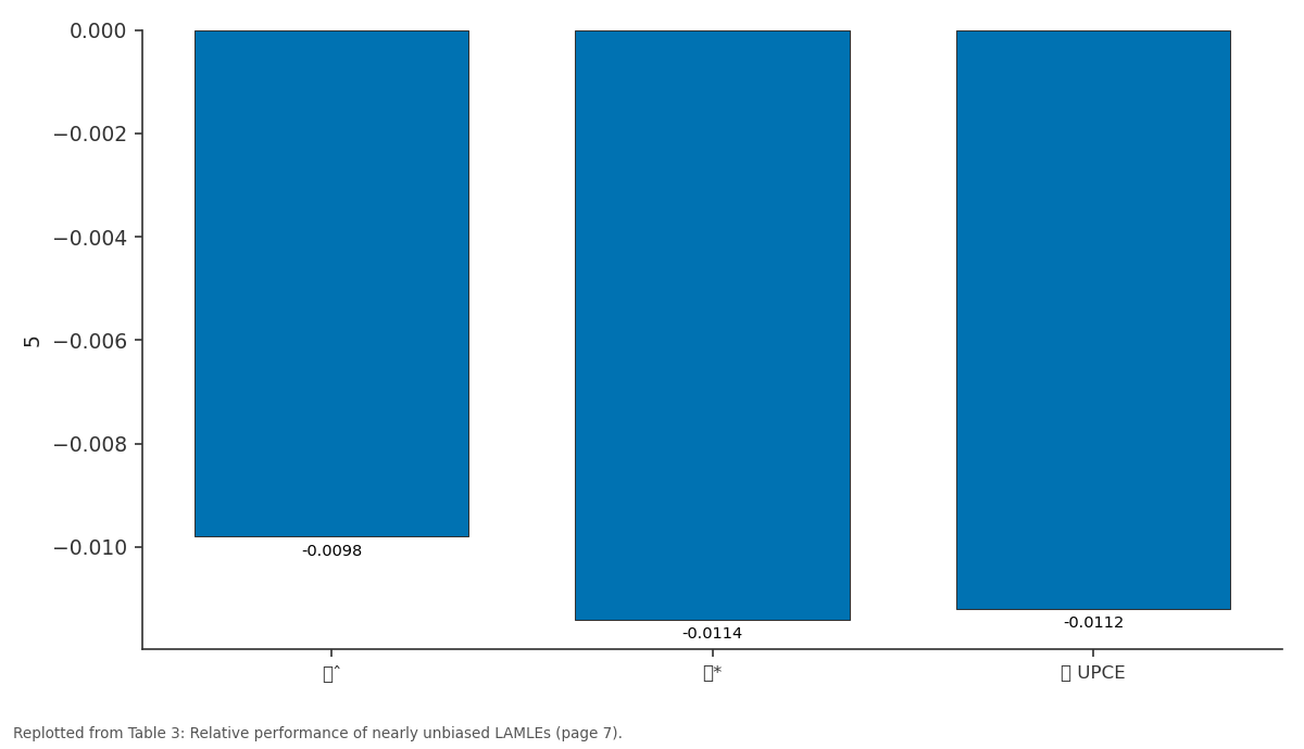
5: ˆ vs * vs UPCE
Replotted from Table 3 (page 7) of the original paper. Every bar is the paper's own table value.
View source evidence ↗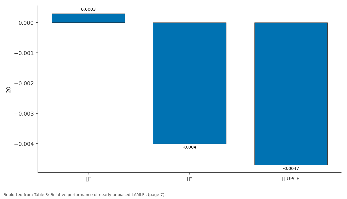
20: ˆ vs * vs UPCE
Replotted from Table 3 (page 7) of the original paper. Every bar is the paper's own table value.
View source evidence ↗Figures & tables
From the original paper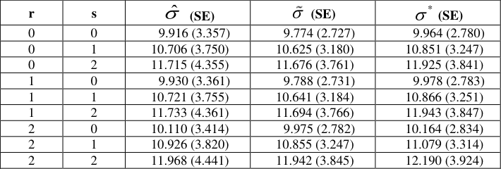 Table 1
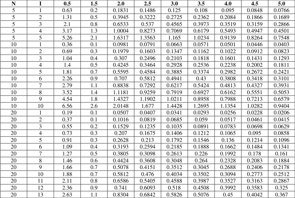 Table 2
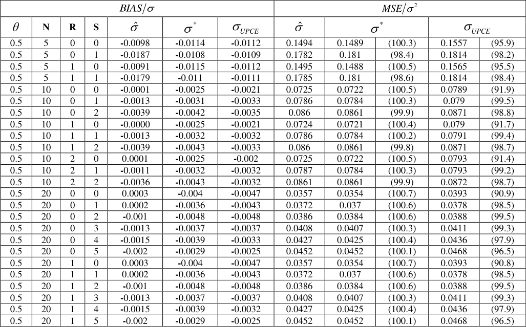 Table 3
Introduction
Consider a series system of components with individually and identically distributed (iid) individual lifetimes, for example, Fx . The reliability function of such a system is given by
; hence, the distribution function of the lifetime random variable of a series system is
Fx as the standard half logistic model, Kantam et al. (2014) [7,11] proposed a new model called the standard Type-II generalized half logistic distribution (GHLD), whose pdf, cdf, and hazard rate function are respectively given by
1 ; 0 x< , 0 . Where is called as the shape parameter. Here, it may be noted that the above standard Type II GHLD is same as the standard Type I GHLD proposed by Olapade (2014) [9] . However, Olapade (2014) [9] derived standard Type I GHLD with a different theoretical argument namely if Y follows an exponential distribution with parameter , then X=log (2e Y -1) is a standard Type I GHLD with parameter .
( ; ) 1
based on Type-II censored samples, by making linear approximations to the intractable terms of the ML equation of σ and we call this estimator as linear approximate MLE (LAMLE). Sec. 3 is devoted for construction of other linear estimator based on percentile method and we call this estimator as percentile estimator (PCE). In Sec. 4, based on a Monte Carlo simulation study, we compare both LAMLE and PCE with the corresponding MLE based on bias and mean square error (MSE). In Sec. 5, we have constructed nearly unbiased LAMLE and nearly unbiased PCE and compare them with the corresponding MLE through a simulation study. An illustrative example is presented in Sec. 6. Finally, in Sec.7, we summarise the conclusions of the study.
Linear Approximate ML Estimation of Scale Parameter Let
is a Type-II censored sample, where r is the number of left most observations censored and s is the number of right most observations censored from a planned sample of size n drawn from the Type II GHLD given in Eq. (1.5). The log-likelihood function of the sample is x the maximum likelihood (ML) equation of , after simplification, is given by 1:
The ML equation (2.2) does not yield explicit solution for because of the presence of the intractable terms
For evaluating the intercepts (α's, γ's) and the slopes (β's, δ's) of the above linear approximations, we have adopted two different linear approximation methods; the first one is based on Taylor series approximation method, which is suggested by Balakrishnan (1989) [1] while studying the approximate ML estimation in scaled Rayleigh distribution and the second one is based on least squares (LS) method, a new approach, suggested by Vasudeva Rao et al. (2017) [13] recently while studying the linear approximate ML estimation in scaled Type I generalised logistic distribution. Upon using the above linear approximations in Eq. (2.2), we get the following approximate ML equation
and solving for , we get a linear estimator of , which we denote as and is given by : 1 ...
of standard Type II GHLD, those are not available in the literature.
Consequently, we are unable to compute the exact mean and exact variance of the LAMLE. However, we have simulated only the means of order statistics of standard Type II GHLD based on 4000 Monte-Carlo runs and tabulated them for n=5, 10, 15 &20. And θ=0.5, 1.5(0.5)5.0 in Table 1. Using these simulated means of order statistics, we can compute approximate mean of for the specified values of n and θ. When sample size n is large, we may use the following approximation for : in a .
| r | s | ˆ (SE) | (SE) | * (SE) |
|---|---|---|---|---|
| 0 | 0 | 9.916 (3.357) | 9.774 (2.727) | 9.964 (2.780) |
| 0 | 1 | 10.706 (3.750) | 10.625 (3.180) | 10.851 (3.247) |
| 0 | 2 | 11.715 (4.355) | 11.676 (3.761) | 11.925 (3.841) |
| 1 | 0 | 9.930 (3.361) | 9.788 (2.731) | 9.978 (2.783) |
| 1 | 1 | 10.721 (3.755) | 10.641 (3.184) | 10.866 (3.251) |
| 1 | 2 | 11.733 (4.361) | 11.694 (3.766) | 11.943 (3.847) |
| 2 | 0 | 10.110 (3.414) | 9.975 (2.782) | 10.164 (2.834) |
| 2 | 1 | 10.926 (3.820) | 10.855 (3.247) | 11.079 (3.314) |
| 2 | 2 | 11.968 (4.441) | 11.942 (3.845) | 12.190 (3.924) |
Table text extracted from the original PDF; superscript letters are shown inline. The original table image is below.
View original table image
The asymptotic variance of can be obtained by inverting the above Fisher information and from which we can compute the standard error of as 11 S.E.( )
By applying Taylor series method to Eq. ( 2.4), we get
Where, i is the i th population quantile of Type II GHLD, given by
Similarly, by applying least squares method (for details of method pl. see Vasudeva Rao et al. (2017) [13] to Eq. (2.4), we get
In the above method, we may take any m≥1. However, Vasudeva Rao et al. (2017) [13] have suggested an optimal choice of m=5, and we have taken the same choice of m.
Thus, in this section, we construct two LAMLEs for based on Type II censored samples using two different linear approximation methods, those are based on the common assumption that the i th standard order statistic Z i:n lies in a narrow neighbourhood of the i th population quantile i . We denote the LAMLEs of computed based on Taylors series method and least squares method respectively by TS and LS .
Percentiles based Estimator of Scale Parameter
Among the most easily obtained estimation methods of the parameters of the Weibull distribution are the graphical approximations to the best linear unbiased estimators. These estimates can be obtained by fitting a straight line to the theoretical points obtained from the distribution function and sample percentile points. This method was originally suggested by Kao (1958, 1959) [5][6] and also see Mann, Schafer and Singpurwalla (1974) [8] and Johnson, Kotz and Balakrishnan (1994) [4] . In case of a Type II GHLD distribution, also it is possible to use same concept to obtain the estimate of based on the percentiles because of the structure of its distribution function. From Eq. (1.5), we have
If i p denotes some estimate of : ;, in Px , then the estimate of can be obtained by minimizing the error sum of squares
Px , then the estimate of can be obtained by minimizing the error sum of squares
It is possible to use several i p 's as estimator of : in Px . However, we use
As explained in the above section, since the variances and covariances of standard Type II GHLD are not available in the literature, we cannot compute exact variance and hence, the standard error of PCE .
Comparison of LAMLE and PCE with MLE
The ML equation (2.2) can be solved iteratively using the well-known Newton-Raphson method, which requires an initial solution of near global maxima. Here, LAMLE can be used as such a good initial solution. We denote MLE, thus obtained, as ˆ.
Like in the case of LAMLE, we cannot obtain the expected Fisher information of MLE. However, we can obtain the observed Fisher information as Where
From which the standard error of is obtained as
In Taylor series and LS methods discussed in the above sections, the basic principle is that the intractable terms [12] . Therefore, the asymptotic variances of exact and approximate MLEs are same (Bhattacharya, 1985). However, the same cannot be said in small samples. At the same time, the small sample bias and variance of MLE are not mathematically tractable. Therefore, we have resorted to Monte Carlo simulation to compute the bias and MSE of , , TS LS and PCE based on 4000 samples of size n=5,10&20 generated from standard Type II GHLD with =0.5,1.5&3.0. We tabulate these simulated biases and MSEs in Table 2.
| N | I | 0.5 | 1.5 | 2.0 | 2.5 | 3.0 | 3.5 | 4.0 | 4.5 | 5.0 |
|---|---|---|---|---|---|---|---|---|---|---|
| 5 | 1 | 0.63 | 0.2 | 0.1831 | 0.1486 | 0.125 | 0.108 | 0.095 | 0.0848 | 0.0766 |
| 5 | 2 | 1.31 | 0.5 | 0.3945 | 0.3222 | 0.2725 | 0.2362 | 0.2084 | 0.1866 | 0.1689 |
| 5 | 3 | 2.1 | 0.8 | 0.6533 | 0.537 | 0.4565 | 0.3973 | 0.3519 | 0.3159 | 0.2866 |
| 5 | 4 | 3.17 | 1.3 | 1.0004 | 0.8273 | 0.7069 | 0.6179 | 0.5493 | 0.4947 | 0.4501 |
| 5 | 5 | 5.26 | 2.1 | 1.6317 | 1.3563 | 1.165 | 1.0234 | 0.9139 | 0.8264 | 0.7548 |
| 10 | 1 | 0.36 | 0.1 | 0.0981 | 0.0791 | 0.0663 | 0.0571 | 0.0501 | 0.0446 | 0.0403 |
| 10 | 2 | 0.69 | 0.3 | 0.1979 | 0.1603 | 0.1347 | 0.1162 | 0.1022 | 0.0912 | 0.0823 |
| 10 | 3 | 1.04 | 0.4 | 0.307 | 0.2496 | 0.2103 | 0.1818 | 0.1601 | 0.1431 | 0.1293 |
| 10 | 4 | 1.4 | 0.5 | 0.4245 | 0.3464 | 0.2928 | 0.2536 | 0.2238 | 0.2002 | 0.1811 |
| 10 | 5 | 1.81 | 0.7 | 0.5595 | 0.4584 | 0.3885 | 0.3374 | 0.2982 | 0.2672 | 0.2421 |
| 10 | 6 | 2.26 | 0.9 | 0.707 | 0.5812 | 0.4941 | 0.43 | 0.3808 | 0.3418 | 0.3101 |
| 10 | 7 | 2.79 | 1.1 | 0.8838 | 0.7292 | 0.6217 | 0.5424 | 0.4813 | 0.4327 | 0.3931 |
| 10 | 8 | 3.52 | 1.4 | 1.1181 | 0.9259 | 0.7919 | 0.6927 | 0.6162 | 0.5551 | 0.5053 |
| 10 | 9 | 4.54 | 1.8 | 1.4327 | 1.1902 | 1.0211 | 0.8958 | 0.7988 | 0.7213 | 0.6579 |
| 10 | 10 | 6.56 | 2.6 | 2.0148 | 1.677 | 1.4428 | 1.2695 | 1.1354 | 1.0282 | 0.9404 |
| 20 | 1 | 0.19 | 0.1 | 0.0507 | 0.0407 | 0.0341 | 0.0293 | 0.0256 | 0.0228 | 0.0206 |
| 20 | 2 | 0.37 | 0.1 | 0.1016 | 0.0819 | 0.0685 | 0.059 | 0.0517 | 0.0461 | 0.0415 |
| 20 | 3 | 0.55 | 0.2 | 0.1529 | 0.1235 | 0.1035 | 0.0891 | 0.0783 | 0.0698 | 0.0629 |
| 20 | 4 | 0.73 | 0.3 | 0.207 | 0.1675 | 0.1406 | 0.1212 | 0.1065 | 0.095 | 0.0858 |
| 20 | 5 | 0.91 | 0.3 | 0.2628 | 0.213 | 0.1792 | 0.1546 | 0.136 | 0.1214 | 0.1096 |
| 20 | 6 | 1.09 | 0.4 | 0.3193 | 0.2594 | 0.2185 | 0.1888 | 0.1662 | 0.1484 | 0.1341 |
| 20 | 7 | 1.27 | 0.5 | 0.3805 | 0.3098 | 0.2613 | 0.226 | 0.1992 | 0.178 | 0.161 |
| 20 | 8 | 1.46 | 0.6 | 0.4424 | 0.3608 | 0.3048 | 0.264 | 0.2328 | 0.2083 | 0.1884 |
| 20 | 9 | 1.66 | 0.7 | 0.5078 | 0.4151 | 0.3512 | 0.3045 | 0.2688 | 0.2406 | 0.2178 |
| 20 | 10 | 1.88 | 0.7 | 0.5812 | 0.476 | 0.4034 | 0.3502 | 0.3094 | 0.2773 | 0.2512 |
| 20 | 11 | 2.11 | 0.8 | 0.6586 | 0.5405 | 0.4588 | 0.3987 | 0.3527 | 0.3163 | 0.2867 |
| 20 | 12 | 2.36 | 0.9 | 0.741 | 0.6093 | 0.518 | 0.4508 | 0.3992 | 0.3583 | 0.325 |
| 20 | 13 | 2.63 | 1.1 | 0.8304 | 0.6842 | 0.5826 | 0.5076 | 0.45 | 0.4042 | 0.367 |
Table text extracted from the original PDF; superscript letters are shown inline. The original table image is below.
View original table image
Nearly Unbiased LAMLE and Nearly Unbiased PCE of scale parameter
While comparing LAMLE with MLE in the above section, we observed that even though LAMLE is almost as efficient as MLE, it is biased than MLE. From Eq. (2.8), we may write
So that σ* is a linear unbiased estimator. Since, we are using simulated : ' in as in place of actual : ' in as , we call σ* as nearly unbiased LAMLE. The asymptotic variance of σ* and hence the standard error of σ* can be obtained as
Where SE is given in Eq (2.10). Similarly, the nearly unbiased percentile estimator of σ, denoted by and are tabulated in Table 3 for Type-II censored samples of size n=5, 10&20 with r=0(1) n/4, s=0(1) n/4 and =0.5, 1.5&3.0. From the table we may conclude that Since the estimators (except MLE) are nearly unbiased, we get negligible simulated biases for the estimators. We may notice that * and UPCE are more biased than when <1, whereas they are less biased than when >1. Thus, when >1, nearly unbiased LAMLE and nearly unbiased PCE are less biased than MLE irrespective of the value of n and amount of censoring whether censoring is left or right or doubly.
| BIAS | — | — | — | — | — | — | MSE 2 | — | — | — | — |
|---|---|---|---|---|---|---|---|---|---|---|---|
| | N | R | S | ˆ | * | UPCE | ˆ | * | UPCE | ||
| 0.5 | 5 | 0 | 0 | -0.0098 | -0.0114 | -0.0112 | 0.1494 | 0.1489 | (100.3) | 0.1557 | (95.9) |
| 0.5 | 5 | 0 | 1 | -0.0187 | -0.0108 | -0.0109 | 0.1782 | 0.181 | (98.4) | 0.1814 | (98.2) |
| 0.5 | 5 | 1 | 0 | -0.0091 | -0.0115 | -0.0112 | 0.1495 | 0.1488 | (100.5) | 0.1565 | (95.5) |
| 0.5 | 5 | 1 | 1 | -0.0179 | -0.011 | -0.0111 | 0.1785 | 0.181 | (98.6) | 0.1814 | (98.4) |
| 0.5 | 10 | 0 | 0 | -0.0001 | -0.0025 | -0.0021 | 0.0725 | 0.0722 | (100.5) | 0.0789 | (91.9) |
| 0.5 | 10 | 0 | 1 | -0.0013 | -0.0031 | -0.0033 | 0.0786 | 0.0784 | (100.3) | 0.079 | (99.5) |
| 0.5 | 10 | 0 | 2 | -0.0039 | -0.0042 | -0.0035 | 0.086 | 0.0861 | (99.9) | 0.0871 | (98.8) |
| 0.5 | 10 | 1 | 0 | -0.0000 | -0.0025 | -0.0021 | 0.0724 | 0.0721 | (100.4) | 0.079 | (91.7) |
| 0.5 | 10 | 1 | 1 | -0.0013 | -0.0032 | -0.0032 | 0.0786 | 0.0784 | (100.2) | 0.0791 | (99.4) |
| 0.5 | 10 | 1 | 2 | -0.0039 | -0.0043 | -0.0033 | 0.086 | 0.0861 | (99.8) | 0.0871 | (98.7) |
| 0.5 | 10 | 2 | 0 | 0.0001 | -0.0025 | -0.002 | 0.0725 | 0.0722 | (100.5) | 0.0793 | (91.4) |
| 0.5 | 10 | 2 | 1 | -0.0011 | -0.0032 | -0.0032 | 0.0787 | 0.0784 | (100.3) | 0.0793 | (99.2) |
| 0.5 | 10 | 2 | 2 | -0.0036 | -0.0043 | -0.0032 | 0.0861 | 0.0861 | (99.9) | 0.0872 | (98.7) |
| 0.5 | 20 | 0 | 0 | 0.0003 | -0.004 | -0.0047 | 0.0357 | 0.0354 | (100.7) | 0.0393 | (90.9) |
| 0.5 | 20 | 0 | 1 | 0.0002 | -0.0036 | -0.0043 | 0.0372 | 0.037 | (100.6) | 0.0378 | (98.5) |
| 0.5 | 20 | 0 | 2 | -0.001 | -0.0048 | -0.0048 | 0.0386 | 0.0384 | (100.6) | 0.0388 | (99.5) |
| 0.5 | 20 | 0 | 3 | -0.0013 | -0.0037 | -0.0037 | 0.0408 | 0.0407 | (100.3) | 0.0411 | (99.3) |
| 0.5 | 20 | 0 | 4 | -0.0015 | -0.0039 | -0.0033 | 0.0427 | 0.0425 | (100.4) | 0.0436 | (97.9) |
| 0.5 | 20 | 0 | 5 | -0.002 | -0.0029 | -0.0025 | 0.0452 | 0.0452 | (100.1) | 0.0468 | (96.5) |
| 0.5 | 20 | 1 | 0 | 0.0003 | -0.004 | -0.0047 | 0.0357 | 0.0354 | (100.7) | 0.0393 | (90.8) |
| 0.5 | 20 | 1 | 1 | 0.0002 | -0.0036 | -0.0043 | 0.0372 | 0.037 | (100.6) | 0.0378 | (98.5) |
| 0.5 | 20 | 1 | 2 | -0.001 | -0.0048 | -0.0048 | 0.0386 | 0.0384 | (100.6) | 0.0388 | (99.5) |
| 0.5 | 20 | 1 | 3 | -0.0013 | -0.0037 | -0.0037 | 0.0408 | 0.0407 | (100.3) | 0.0411 | (99.3) |
| 0.5 | 20 | 1 | 4 | -0.0015 | -0.0039 | -0.0032 | 0.0427 | 0.0425 | (100.4) | 0.0436 | (97.9) |
| 0.5 | 20 | 1 | 5 | -0.002 | -0.0029 | -0.0025 | 0.0452 | 0.0452 | (100.1) | 0.0468 | (96.5) |
Table text extracted from the original PDF; superscript letters are shown inline. The original table image is below.
View original table image
In moderate and large samples (n>10), * is performing remarkably with more than 99% efficiency as compared with irrespective of the amount of censoring whether it is left censoring or right censoring or doubly censoring. Even in small samples (n<10), it is performing with a minimum of 95% efficiency. Though UPCE is as good as * in terms of bias, it is not as efficient as * in terms of MSE.
For >1, except in small samples (n<10), *
is not only performing with more than 97% efficiency, but also less biased than MLE. Therefore, unbiased LAMLE is preferable to MLE in these cases. Remark: In the above, σ* is computed using least squares method. However, we will get the same conclusions even if we use Taylor series method.
Illustration
We consider the following sorted sample of size 10, which is simulated from Type II GHLD with =10 and =3. 0.07, 0.50, 2.90, 4.99, 5.02, 6.46, 8.06, 8.93, 9.46, 10.52.
We have computed ˆ, and * and for the above sample with different choices of r and s and tabulated below. Here, for computation of and * , we have used least squares method. Since, PCE and UPCE are not so efficient, we have not computed them.
The standard errors of ˆ, and * are computed from Eqs. (4.3), (2.10) and (5.2) respectively, which are derived based on Fisher information of the estimators. From the above table, we may notice that the standard error MLE is larger than that of LAMLE, perhaps, this is due to the fact that the former is based on observed Fisher information whereas the latter is based on expected Fisher information. Even though, the standard error of is slightly smaller than that of * , * is better than , since * is the bias reduced estimator.
References
13 in the original paper- Balakrishnan N. Approximation MLE of scale parameter of the Rayleigh distribution with censoring. IEEE Transactions on Reliability. 1989; (38):355-357.
- Bhattacharya GK. The asymptotic of maximum likelihood and related estimators based on Type-II censored data. JASA. 1985; (80):398-404.
- Devendra Kumar, Neetu Jain, Shivani Gupta. The Type I Generalized Half-Logistic Distribution Based on Upper Record Values. Journal of Probability and Statistics. 2015, 1-11.
- Johnson NL, Kotz S, Balakrishnan N. Continuous Univariate Distribution. 2 nd edition, New York, Wiley, 1994, 1.
- Kao JHK. Computer methods for estimation Weibull parameters in reliability studies. Transaction of IRE-Reliability and Quality control. 1958; 13:15-22.
- Kao JHK. A graphical estimation of mixed Weibull parameters in reliability studies. Technometrics. 1959; 1:389-407.
- Kantam RRL, Ramakrishna V, Ravikumar MS. Estimation and testing in type 1 generalized half logistic distribution. Modern applied statistical methods. 2014; 12(1):198-206.
- Mann Schafer RE, Singpurwalla ND. Methods for Statistical Analysis of Reliability and Life Data. New York, Wiley, 1974.
- Olapade AK. The type I generalized half logistic distribution. Journal of the Iranian Statistical Society. 2014; 13(1):69-82.
- Phillip Oluwatobi Awodutiristice, Akintayo Kehinde Olapade, Oladapo Adedayo Kolawole. The Type I Generalized Half Logistic Survival Model. International Journal of Theoretical and Applied Mathematics. 2016; 2(2):74-78.
- Rosaiah K, Kantam RRL, Rama Krishna V. Type-II Generalized Half Logistic Distribution-An Economic Reliability Test Plan. Journal of Chemical, Biological and Physical Sciences. 2014; 4(1):501-508.
- Tiku ML, Tan WY, Balakrishnan N. Robust Inference, New York: Marcel Dekker, 1986.
- Vaudeva Rao A, Sitaramacharyulu P, ChenchuRamaiah M. Linear approximate ML estimation in scaled Type I generalized logistic distribution based on Type-II censored samples. Commun. Statist-Simul. Comput. 2017; 46(3):1682-1702.
Cited by 1
From OpenAlex, OpenCitations and reference lists read by Scinovex
- Designing of multiple dependent state sampling plan for Type-II generalized half logistic distribution ↗
Sd. Jilani, Gadde Srinivasa Rao, A. V. Dattatreya Rao · Research in Mathematics · 2024
In this study, we propose the multiple dependent state (MDS) sampling plan for a time truncated life test when the lifetime of product follows the Type-II Generalized Half Logistic Distribution (TGHLD). The quality of the product is considered in terms of percentile lifetime. The optimal plan parameters of the our proposed MDS sampling plan, such as the sample size, the…
❝ 2PDF