
Research article · 2018 · Full text
International Journal of Statistics and Applied MathematicsComparison of shared frailty models: A Bayesian approach
Volume 3(2) · Pages 511–517
Research areasInsurance, Mortality, Demography, Risk Management
Abstract
Author-writtenIn this article, we propose gamma and inverse Gaussian frailty shared models with Akash distribution as baseline to analyze the bivariate survival data set of Mc Gilchrist and Aisbett (1991). Bayesian approach of Markov Chain Monte Carlo technique was employed to estimate the parameters involves in the models. The better model also suggested for the data.
Summary
Source-checkedPlain-language reading of the full paper, prepared with AI and checked against the text. Each point links to the authors' own words.
Why it matters
- The Cox proportional hazard model is a standard method in survival analysis, though it assumes the study population is homogeneous. View evidence ↗
- Frailty refers to unobserved covariates that account for heterogeneity within a population. View evidence ↗
- Using frailty allows researchers to incorporate random effects and dependence into survival data models. View evidence ↗
The question
- The study aims to compare a shared gamma frailty model, a shared inverse Gaussian frailty model, and a model without frailty (Cox proportional hazard model) using a Bayesian approach. View evidence ↗
What they did
- The researchers used the Akash distribution, a modification of the Lindley distribution, as the baseline distribution for their models. View evidence ↗
- The models were tested using kidney infection recurrence data from 38 patients using portable dialysis equipment. View evidence ↗
- The Bayesian models were fitted using Markov Chain Monte Carlo (MCMC) methods, specifically the Metropolis-Hastings algorithm. View evidence ↗
- Model comparison was performed using AIC, BIC, DIC, and the Bayes factor. View evidence ↗
What they found
- Goodness-of-fit tests showed no statistical evidence to reject the hypothesis that the recurrence times follow the proposed frailty distributions. View evidence ↗
- Frailty models (Model-I and Model-II) performed better than the model without frailty (Model-III), as indicated by lower AIC, BIC, and DIC values. View evidence ↗
- Bayes factor analysis showed that Model-II was superior to Model-I (Djk = 5.4129) and Model-III (Djk = 27.2213). View evidence ↗
- High frailty variance estimates (1.2647 for gamma and 1.9016 for inverse Gaussian) suggest significant heterogeneity among the patients. View evidence ↗
What it means
- The authors conclude that the inverse Gaussian frailty model with an Akash baseline distribution is the most effective for modeling kidney infection data. View evidence ↗
- The authors state that both shared gamma and shared inverse Gaussian frailty models are superior to models without frailty for this dataset. View evidence ↗
Visual summary
1 visualsIllustrations explain the paper; charts are replotted from the paper's own table values.
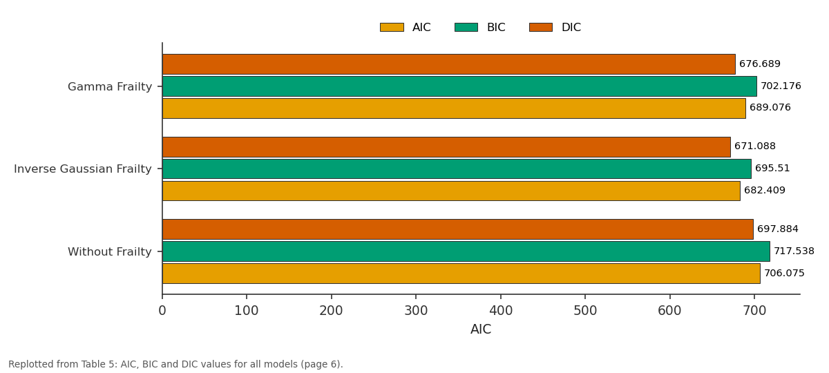
AIC and BIC and more: Gamma Frailty vs Inverse Gaussian Frailty vs Without Frailty
Replotted from Table 5 (page 6) of the original paper. Every bar is the paper's own table value.
View source evidence ↗Figures & tables
From the original paper Table 1
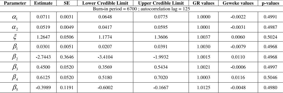 Table 2
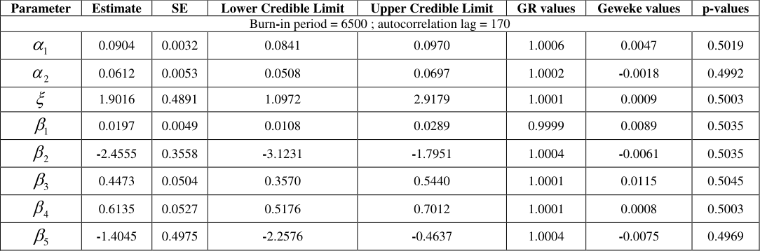 Table 3
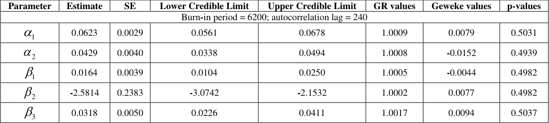 Table 3
 Table 5
 Table 5
 Table 6
Introduction
In survival analysis Cox proportional hazard model by Cox (1972) [2] is the most commonly used method. It is assumed that the study population is homogeneous. But In many applications, consider populace cannot be expected to be homogeneous but must be considered as a heterogeneous sample, i.e. a blend of people with different hazards. For illustration, in many cases it is possible to include all the covariates related to the illness of interest due to economical reasons or sometimes the significance of a few covariates is still obscure. The missing or unobserved covariate is termed as "frailty" which account for heterogeneity in the population. The notion of frailty provides a convenient way to introduce random effects, dependence and unobserved heterogeneity into models for survival data. The term frailty itself was introduced by Vaupel et al. (1979) [14] in univariate survival models and the model was substantially promoted by its application to multivariate survival data in a seminal paper by Clayton (1978) [1] (without using the notion "frailty") on chronic disease incidence in families. The frailty approach could be a statistical modeling concept which points to account for heterogeneity, caused by unmeasured covariates. In statistical terms, a frailty model may be a random effect model for time-to-event data, where the random effect (the slightness) features a multiplicative impact on the baseline hazard function. Hanagal (2007) [3] proposed gamma frailty regression models in mixture distribution. Hangal and Shama (2013) [7] also suggested gamma shared frailty for modeling heterogeneity in bivariate survival data. Hanagal and Pandey (2017) [6] considered inverse Gaussian distribution as frailty parameter and compared the models by using kidney infection data. In this manuscript, we compare shared gamma frailty model, shared inverse Gaussian frailty model and the model without frailty i.e. Cox proportional hazard model by using Bayesian method of comparison.
Baseline distribution
The baseline distribution used here is Akash Distribution proposed by Shanker (2015) [13] , which is the modification of Lindley distribution (Lindley, 1958) [11] . Akash distribution is able to fit in data obtained from medical sciences and engineering.
A continuous random variable T is said to follow the Akash distribution with the parameter if its survival function is,
And the hazard function and the cumulative hazard function as 2 (1 ) ()
The hazard function is increasing and more flexible than Lindley distribution and exponential distribution. That is why we choose as baseline distribution.
Proposed Models
Substituting the cumulative hazard function in equations (2.5), (2.7) and (2.8), we get the unconditional survival function of bivariate random variable (T 1j , T 2j ), then
Equations (4.1) and (4.2) are gamma shared frailty and inverse Gaussian shared frailty models with baseline Akash distribution and called as model-I and model-II, equation (4.3) is without frailty with baseline Akash distribution and called as model-III.
Methodology
The likelihood function associated with the failures times and censoring variables ij (i =1,2; j = 1,2,…n) based on the survival function is given as
International Journal of Statistics and Applied Mathematics Where , and are the vector of baseline parameter, the vector of regression coefficients, and the frailty parameter. For without frailty model likelihood function is
Substituting distribution function S (t 1j , t 2j ) and by differentiating we get the likelihood function given by equation (5.1). Similarly we get the likelihood function for without frailty model. The likelihood function obtained in equation (5.1) is not easy to solve since it involves a large number of parameters in the model by using Newton-Raphson method, the MLEs is not converge. Thus, we move to the Bayesian approach, which does not suffer any kind of such difficulties. The joint posterior density function of parameters for given failure times is obtained as,
Where g i (.) (i = 1, 2, 3) indicates the prior density function with known hyper parameters of corresponding arguments for baseline parameters and frailty variance; p i (.) is prior density function for regression coefficient β i and likelihood function L (.) is given by equation (5.1) or (5.2). Here we assume that all the parameters are independently distributed. The non-informative prior was used for frailty parameters and regression coefficients. Since we do not have prior information on baseline parameters, it is assumed to be flat. The prior distribution for the parameters used is as follows-For frailty parameter ( ) ~ (0.0001, 0.0001)
For regression coefficients ( ) ~ Normal (0, 1000)
For baseline parameters ( ) ~ (1, 0.0001) and U (0, 100)
We have fitted the Bayesian model with the above prior density functions and likelihood function (5.1) using the MCMC methods such as, the Metropolis-Hastings algorithm. We have monitored convergence of Markov chain to a stationary distribution by Gelman-Rubin convergence statistic and Geweke test. Trace plots, coupling from the past plots and sample autocorrelation function plots have been used to check the behavior of the chain, to decide burn-in period and sample autocorrelation lag respectively.
In order to compare the proposed models we have used several Bayesian model selection criteria such as, Bayesian Information Criteria (BIC), Akaike Information Criteria (AIC) and Deviance Information Criteria (DIC). Also we have used the Bayes factor B jk for comparison of the modelsM j against M k . To compute the Bayes factor we have considered MCMC approach given in Kass and Raftery (1995) [9] .
Data Analysis
Kidney infection data of McGrilchrist and Aisbett (1991) [12] was utilized demonstrate the Bayesian estimation technique. The data are comprises of infection recurrence times at the point of insertion of the catheter for 38 kidney patients using portable dialysis equipment. For each patient, the occurrences of infection for the first and second time were recorded. It may be removed other than infection and regarded as censoring. So the first or second infection time or censoring time may be the survival times.
To cure the first infection sufficient time was permitted before the catheter was inserted for the second time. So the first and second recurrence times are taken to be independent apart from the common frailty component. The data of the risk variables are age, sex and disease type GN, AN and PKD where GN, AN and PKD are brief forms of Glomerulo Neptiritis, Acute Neptiritis and Polycystic Kidney Disease.
Let T 1 and T 2 be the first and the second recurrence time to infection. Five covariates age, sex and presence or absence of disease type GN, AN and PKD are represented by X 1 , X 2 , X 3 , X 4 , and X 5 .
First we check goodness of fit to the data for frailty models and then apply the Bayesian estimation procedure. Kolmogorov-Smirnov test was considered to check goodness of fit for the kidney infection data set test and the p-values also obtained for T 1 and T 2 separately. Corresponding p-values are displayed in Table 1.
| Model | Recurrences times | — |
|---|---|---|
| First | Second | |
| Gamma frailty | 0.9024 | 0.3720 |
| Inverse Gaussian Frailty | 0.4490 | 0.1229 |
Table text extracted from the original PDF; superscript letters are shown inline. The original table image is below.
View original table image
Figures and tables from the paper
| Baseline distribution | Model | AIC | BIC | DIC | Log-likelihood |
|---|---|---|---|---|---|
| Akash Distribution | Gamma Frailty | 689.0755 | 702.1761 | 676.6887 | -336.5377 |
| Inverse Gaussian Frailty | 682.4093 | 695.5100 | 671.0884 | -333.2046 | |
| Without Frailty | 706.0754 | 717.5385 | 697.8843 | -346.0377 |
Table text extracted from the original PDF; superscript letters are shown inline. The original table image is below.
View original table image
| Numerator model against denominator model | Djk=2loge(Bij) | range | Evidence against model in denominator |
|---|---|---|---|
| II against I | 5.4129 | ≥2 and ≤6 | Positive |
| II against III | 27.2213 | ≥ 10 | Very strong positive |
| I against III | 21.8083 | ≥ 10 | Very strong positive |
Table text extracted from the original PDF; superscript letters are shown inline. The original table image is below.
View original table image
References
14 in the original paper- Clayton DG. A model for association in bivariate life tables and its application in epidemologicalstudies of familial tendency in chronic diease incidence, Biometrika. 1978; 65:141-151.
- Cox DR. Regression models and life tables (with discussion), Journal of the Royal Statistical Society B. 1972; 34:187-220.
- Hanagal DD. Gamma frailty regression models in mixture distributions. Economic Quality Control. 2007; 22(2):295-302.
- Hanagal DD, Dabade AD. Modelling heterogeneity in bivariate survival data by compound Poisson distribution using Bayesian approach. International Journal of Statistics and Management Systems. 2012; 7(1):36-84.
- Hanagal DD, Dabade AD. Bayesian estimation of parameters and comparison of shared gamma frailty models. Communications in Statistics-Simulation and Computation. 2013; 42 (4):910-931.
- Hanagal DD, Pandey A. Shared inverse Gaussian frailty models based on additive hazards. Communications in StatisticsTheory and Methods. 2017; 46(22):11143-11162.
- Hanagal DD, Sharma R. Modeling heterogeneity for bivariate survival data by shared gamma frailty regression model. Model Assisted Statistics and Applications. 2013; 8(2):85-102.
- Hougaard P. Life table methods for heterogeneous populations. Biometrika. 1984; 71(1):75-83.
- Kass RE, Raftery AE, Bayes factor. Journal of the American Statistical Association. 1995; 90(430):773-795.
- Kheiri S, Kimber A, Meshkani MR. Bayesian analysis of an inverse Gaussian correlated frailty model. Computational Statistics and Data Analysis. 2007; 51:5317-5326.
- Lindley DV. Fiducial distributions and Bayes' theorem, Journal of the Royal Statistical Society, Series B. 1958; 20:102-107.
- McGilchrist CA, Aisbett CW. Regression with frailty in survival analysis. Biometrics. 1991; 47:461-466.
- Shanker R. Akash distribution and its applications. International journal of probability and Statistics. 2015; 4(3):67-75.
- Vaupel JW, Manton KG, Stallard E. The impact of heterogeneity in individual frailtyon the dynamics of mortality. Demography. 1979; 16:439-454.
Cited by 1
From OpenAlex, OpenCitations and reference lists read by Scinovex
- Posterior consistency in frailty models and simulation studies to test the presence of random effects ↗
Gwangsu Kim · Journal of the Korean Statistical Society · 2018
❝ 1