
Research article · 2020 · Full text
International Journal of Statistics and Applied MathematicsAn economic reliability test plan for exponentiated half logistic distributed lifetimes
Volume 5(2) · Pages 140–148
Research areasStatistical Distribution Estimation and ApplicationsReliability and Maintenance OptimizationAdvanced Statistical Process Monitoring
Abstract
Author-writtenThe exponentiated half logistic distribution introduced by Cordeiro et al. (2014) is a probability model for the life time of an item. A submitted lot will be accepted or rejected based on the sampling plans where items are to be tested and for collecting the life of items, these plans are called reliability test plans. The present reliability test plan is more desirable than similar plans exists in literature is entrenched with respect to termination time of the experiment. For a range of stated acceptance number we determine the minimum life test termination time, sample size, and producer’s risk.
Summary
Source-checkedPlain-language reading of the full paper, prepared with AI and checked against the text. Each point links to the authors' own words.
Why it matters
- Reliability studies are essential in quality control because they allow researchers to reduce the time and cost associated with deciding whether to accept or reject a submitted lot of items. View evidence ↗
- Reliability testing involves managing two types of errors: producer's risk (type-I error), where good items are rejected, and consumer's risk (type-II error), where bad items are accepted. View evidence ↗
- Skewed or asymmetrical probability distributions are often used to create reliability sampling plans that are more cost-effective for researchers. View evidence ↗
The question
- The authors aim to establish economic reliability test plans specifically based on the exponentiated half logistic distribution (EHLD). View evidence ↗
What they did
- The authors calculated minimum sample sizes for various shape parameters (ν = 2, 3, and 1.1358) and risk probabilities (α = 0.75, 0.90, 0.95, 0.99) with r ranging from 1 to 10. View evidence ↗
- To illustrate the plan, the authors used real lifetime data regarding vinyl chloride concentrations in ground-water monitoring wells. View evidence ↗
What they found
- The vinyl chloride data set was found to fit the EHLD reasonably well, with a Kolmogorov-Smirnov statistic of 0.1192 and a p-value of 0.719. View evidence ↗
- Using an existing sampling plan (n=5, c=0, ratio=0.90) on the real data, the product was rejected because four readings were below the 0.36 µg/L threshold. View evidence ↗
- The proposed plan is preferred because it reaches a decision at a lower ratio (0.0356 vs 0.90), resulting in less waiting time and lower experimental costs. View evidence ↗
What it means
- The authors conclude that their proposed plan minimizes the ratio of termination time needed to decide whether to accept or reject a lot. View evidence ↗
- The authors state that the proposed plan is effective in minimizing the producer's risk. View evidence ↗
Figures & tables
From the original paper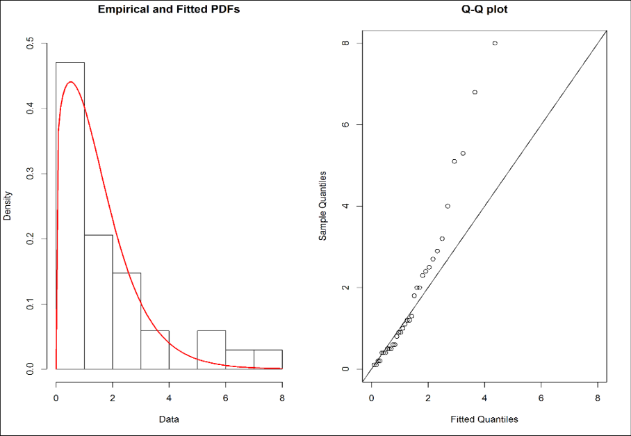 Figure 1
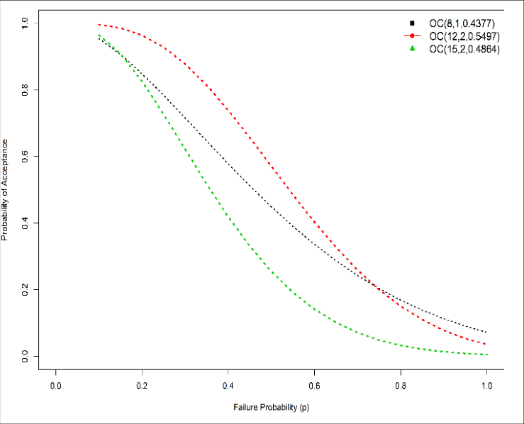 Figure 2
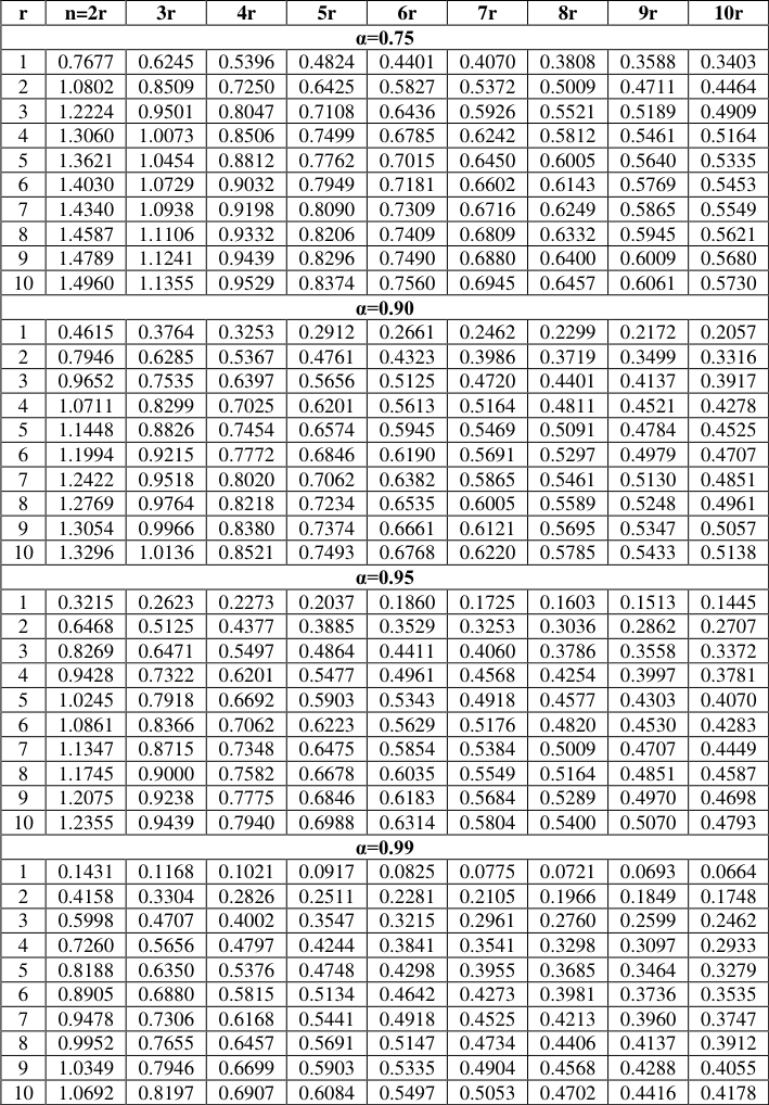 Table 1
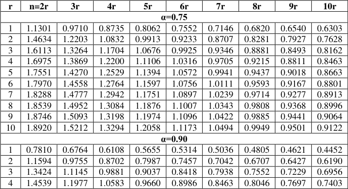 Table 2
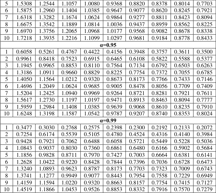 Table 3
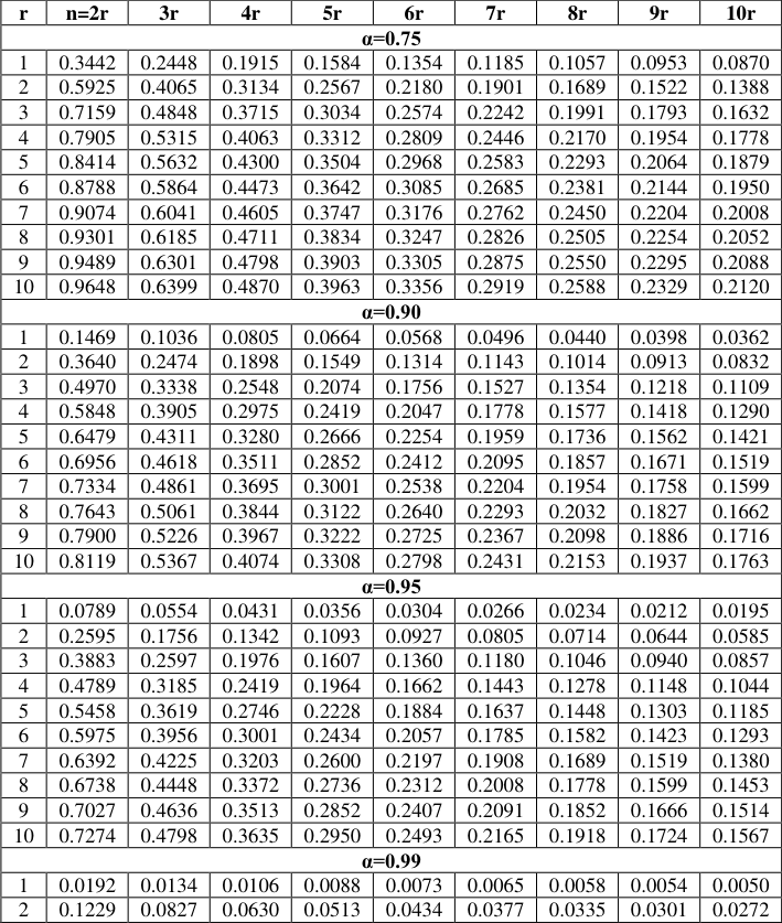 Table 3
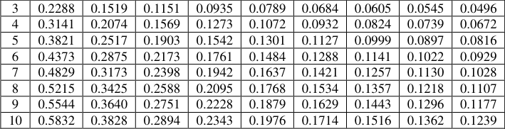 Table 4
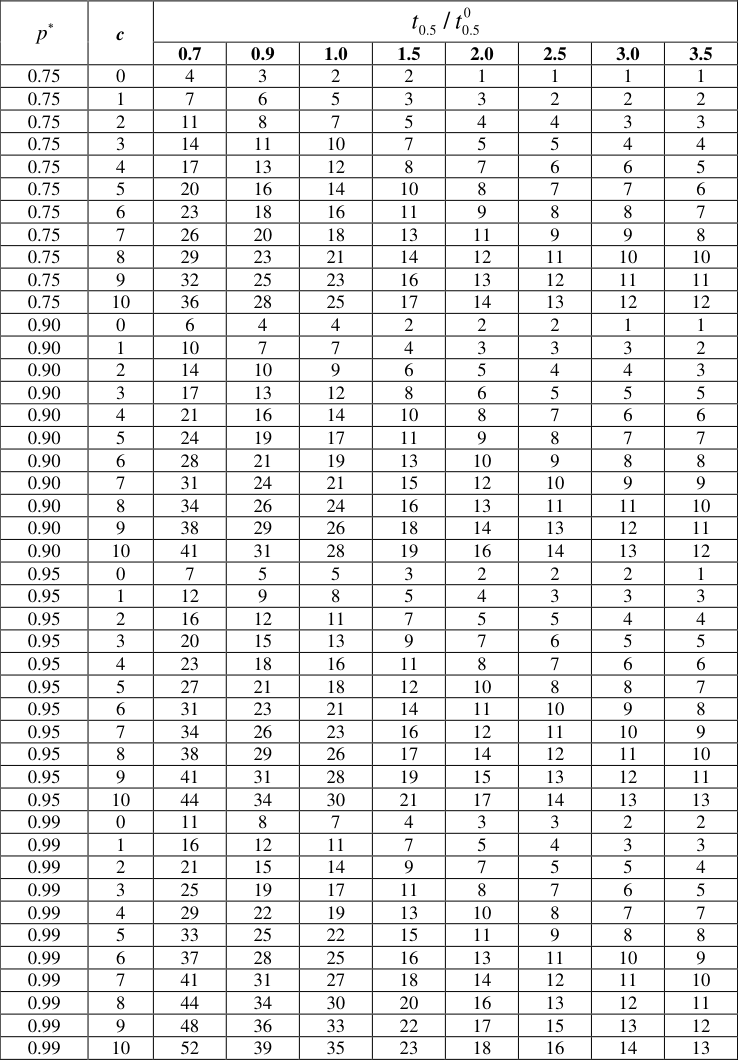 Table 4
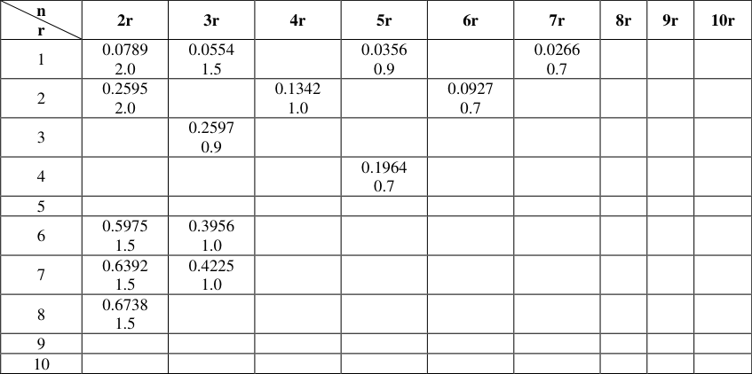 Table 5
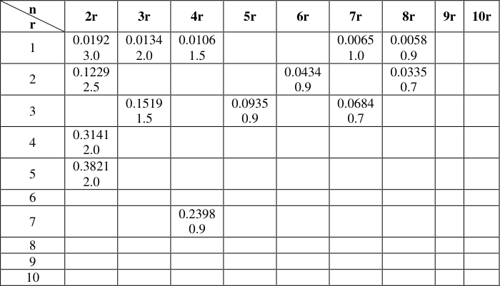 Table 6
Introduction
In quality control the study of reliability play a key role. The researcher can minimize the time and cost in the process of accepting or rejecting the submitted lot on the basis of reliability study. If the unpretentious items will be rejected based on the sample information, which is called type-I error (producer's risk ). On the contrary, if the unpretentious items will be accepted, which is called type-II error (consumer's risk ). The procedure of acceptance or rejection of the lot conditional upon the risks related with two types of errors is known as 'reliability test plan' or 'acceptance sampling based on life test'; for further details, see Duncan (1986) [7] and Stephens (2001) [24] . Asymmetrical probability distributions are the basis for reliability test plans. The reliability sampling plans which are more cost-effective for the researcher used to found by skewed distributions. The truncated life tests in exponential distribution was first contemplated by Epstein and Sobel (1954) [8] . The median is a preferable quality parameter than the mean which was suggested by Gupta (1962) [9] . On the contrary, the mean is better parameter for symmetrical distributions. The acceptance sampling plans will be used for the quantiles suggested by Balakrishnan et al. (2007) [4] and also derived the formulae. The generalized exponential distribution was contemplated to justify economic reliability test plan by Aslam and Shahbaz (2007) [3] . The economic reliability test plan for a generalized Rayleigh Distribution was also presented by Aslam (2008) [1] . The need of engineering on the definite percentile of strength or breaking stress may not be satisfied by the acceptance sampling plans based on mean suggested by Lio et al. (2009, 2010) [14,15] and they also suggested that the acceptance sampling plans based on the truncated life tests to Birnbaum-Saunders distribution and Burr type XII for percentiles. The economic reliability group acceptance sampling plans for lifetimes of Marshall-Olkin extended distribution introduced by Mugahal et al. (2010) [16] . The economic reliability group acceptance sampling plan for Pareto second kind distribution conferred by Aslam et al. (2010) [2] . The economic reliability test plan on the basis of Marshall-Olkin extended exponential distribution described by Rao et al. (2011) [18] . The reliability test plans for type-II exponentiated log-logistic distribution was conferred by Rao et al. (2012) [19] . The economic reliability test plan for a generalized log-logistic distribution presented by Rao et al. (2013) [20] . The acceptance sampling plans based on median life for Fréchet distribution was developed by Balamurali et al. (2013). The economic reliability test plan based on truncated life tests for Marshall-Olkin extended Weibull Distribution was considered by Rao (2015) [17] . The economic reliability test plan for Type-I and Type-II generalized half logistic distribution was considered by Rosaiah et al. (2014a, 2014b) [22,23] . Under the reliability test plans the test termination time can be determined. The probability distributions/models have been in use to evolve the reliability test plans. The best reliability sampling plans which are more inexpensive for the researcher can be determined using these probability distributions. The log-logistic distribution to develop the acceptance sampling plans could be used by Kantam et al. (2001). Also studied the reliability test plans using the log-logistic distribution by Kantam et al. (2006) [11] . The experiment will be terminated in reliability test plan if the th r failure occurs if we put the nr sample units on test or if the termination time t ends, whichever occurs first.
In this paper we establish the economic reliability test plans based on exponentiated half logistic distribution (EHLD) with reference to the above cited economic reliability test plans for various distributions. In Unit 2, we define briefly about the EHLD. The plan of the suggested economic reliability test plans is conferred in in Unit 3. In Unit 4, we describe the proposed design and attain the required results and illustrative example with real data is also provided. Finally, in Unit 5 conclusions are made.
The Exponentiated Half Logistic Distribution
Let us consider the life time of an item follows the exponentiated half logistic distribution (EHLD). The EHLD was established and studied quite extensively by Cordeiro et. al. (2014). The probability density function (pdf), cumulative distribution function (cdf) and hazard function (hf) of EHLD are respectively given as follows:
Where, σ is the scale parameter and is shape parameter.
An Economic Reliability Test Plan for EHLD
The minimum sample size needed to establish a percentile life when the observed number of failures does not exceed a given acceptance number c and when the test is terminated at a pre-assigned time 0 q t was obtained and also to make decision about the submitted lot, the minimum sample sizes required are determined by Rao and Ramesh Naidu (2014) [21] for the given acceptance number c , the waiting time in terms of 0 q t (i.e., 0 / q t t ), and some risk probability, say , based on the median/percentile for EHLD. The conservation to the consumer is provided by the procedure of accepting the lot only if the specified percentile of lifetime can be established with a pre-assigned high probability . The brief contents of Rao and Ramesh Naidu (2014) [21] are
given for the reference. The minimum sample size 'n' can be determined for spedific values of (0 < < 1), 0 / q t t , for a specified 0 q t of q t and the acceptance number c such that 0 (1 )
given by eqn. (2) which designates the failure probability before time t, and depends on the ratio 0 / q q t t . It is appropriate to stipulate this ratio for designing the experiment.
Rao and Ramesh Naidu (2014) [21] obtained the minimum values of n satisfying the inequality (4) for =2, =0.75, 0.90, 0.95, 0.99 and 0 / q q t t =0.7, 0.9, 1.0, 1.5, 2.0, 2.5, 3.0, 3.5 which are provided in Table-4 for ready reference.
The inequality ( 4) is presented in different way in the current study. Let the sample size n is fixed and r ( n ) be a natural number, the process will be stopped and the lot is rejected as soon as the ) 1 ( c r r th failure occurs. The probability that the rejection of that lot must be as small as possible for the given q t > 0 q t and it is given by: (1 ) 1
The inequality (5) can be viewed as an inequality in an unknown quantity 0 / q q t t with known parameter by taking n as a multiple of r say kr ( k =1, 2 …). The inequality (5) will be solved for the smallest p say 0 p from which the value of . These values are provided in Table 1 for different values of n , r =1(1)10, =2 at =0.75, 0.90, 0.95, 0.99 and Table 2 andTable 3 provide different values of r =1(1)10 for =3 and the estimated values =1.1358 respectively at =0.75, 0.90, 0.95, 0.99 and also Table -5 andTable-6 provided the comparison between Rao and Ramesh Naidu (2014) [21] and the current smpling plan for =0.95 and 0.99.
| r | n=2r | 3r | 4r | 5r | 6r | 7r | 8r | 9r | 10r |
|---|---|---|---|---|---|---|---|---|---|
| α=0.75 | |||||||||
| 1 | 1.1301 | 0.9710 | 0.8735 | 0.8062 | 0.7552 | 0.7146 | 0.6820 | 0.6540 | 0.6303 |
| 2 | 1.4634 | 1.2203 | 1.0832 | 0.9913 | 0.9233 | 0.8707 | 0.8281 | 0.7927 | 0.7628 |
| 3 | 1.6113 | 1.3264 | 1.1704 | 1.0676 | 0.9925 | 0.9346 | 0.8881 | 0.8493 | 0.8162 |
| 4 | 1.6975 | 1.3869 | 1.2200 | 1.1106 | 1.0316 | 0.9705 | 0.9215 | 0.8811 | 0.8463 |
| 5 | 1.7551 | 1.4270 | 1.2529 | 1.1394 | 1.0572 | 0.9941 | 0.9437 | 0.9018 | 0.8663 |
| 6 | 1.7970 | 1.4558 | 1.2764 | 1.1597 | 1.0756 | 1.0111 | 0.9593 | 0.9167 | 0.8801 |
| 7 | 1.8288 | 1.4777 | 1.2942 | 1.1751 | 1.0897 | 1.0239 | 0.9714 | 0.9277 | 0.8913 |
| 8 | 1.8539 | 1.4952 | 1.3084 | 1.1876 | 1.1007 | 1.0343 | 0.9808 | 0.9368 | 0.8996 |
| 9 | 1.8746 | 1.5093 | 1.3198 | 1.1974 | 1.1096 | 1.0422 | 0.9885 | 0.9441 | 0.9064 |
| 10 | 1.8920 | 1.5212 | 1.3294 | 1.2058 | 1.1173 | 1.0494 | 0.9949 | 0.9501 | 0.9122 |
| α=0.90 | |||||||||
| 1 | 0.7810 | 0.6764 | 0.6108 | 0.5655 | 0.5314 | 0.5036 | 0.4805 | 0.4621 | 0.4452 |
| 2 | 1.1594 | 0.9755 | 0.8702 | 0.7987 | 0.7457 | 0.7042 | 0.6707 | 0.6427 | 0.6190 |
| 3 | 1.3424 | 1.1145 | 0.9881 | 0.9037 | 0.8418 | 0.7938 | 0.7552 | 0.7229 | 0.6956 |
| 4 | 1.4539 | 1.1977 | 1.0583 | 0.9660 | 0.8986 | 0.8463 | 0.8046 | 0.7697 | 0.7403 |
Table text extracted from the original PDF; superscript letters are shown inline. The original table image is below.
View original table image
| r | n=2r | 3r | 4r | 5r | 6r | 7r | 8r | 9r | 10r |
|---|---|---|---|---|---|---|---|---|---|
| α=0.75 | |||||||||
| 1 | 0.7677 | 0.6245 | 0.5396 | 0.4824 | 0.4401 | 0.4070 | 0.3808 | 0.3588 | 0.3403 |
| 2 | 1.0802 | 0.8509 | 0.7250 | 0.6425 | 0.5827 | 0.5372 | 0.5009 | 0.4711 | 0.4464 |
| 3 | 1.2224 | 0.9501 | 0.8047 | 0.7108 | 0.6436 | 0.5926 | 0.5521 | 0.5189 | 0.4909 |
| 4 | 1.3060 | 1.0073 | 0.8506 | 0.7499 | 0.6785 | 0.6242 | 0.5812 | 0.5461 | 0.5164 |
| 5 | 1.3621 | 1.0454 | 0.8812 | 0.7762 | 0.7015 | 0.6450 | 0.6005 | 0.5640 | 0.5335 |
| 6 | 1.4030 | 1.0729 | 0.9032 | 0.7949 | 0.7181 | 0.6602 | 0.6143 | 0.5769 | 0.5453 |
| 7 | 1.4340 | 1.0938 | 0.9198 | 0.8090 | 0.7309 | 0.6716 | 0.6249 | 0.5865 | 0.5549 |
| 8 | 1.4587 | 1.1106 | 0.9332 | 0.8206 | 0.7409 | 0.6809 | 0.6332 | 0.5945 | 0.5621 |
| 9 | 1.4789 | 1.1241 | 0.9439 | 0.8296 | 0.7490 | 0.6880 | 0.6400 | 0.6009 | 0.5680 |
| 10 | 1.4960 | 1.1355 | 0.9529 | 0.8374 | 0.7560 | 0.6945 | 0.6457 | 0.6061 | 0.5730 |
| α=0.90 | |||||||||
| 1 | 0.4615 | 0.3764 | 0.3253 | 0.2912 | 0.2661 | 0.2462 | 0.2299 | 0.2172 | 0.2057 |
| 2 | 0.7946 | 0.6285 | 0.5367 | 0.4761 | 0.4323 | 0.3986 | 0.3719 | 0.3499 | 0.3316 |
| 3 | 0.9652 | 0.7535 | 0.6397 | 0.5656 | 0.5125 | 0.4720 | 0.4401 | 0.4137 | 0.3917 |
| 4 | 1.0711 | 0.8299 | 0.7025 | 0.6201 | 0.5613 | 0.5164 | 0.4811 | 0.4521 | 0.4278 |
| 5 | 1.1448 | 0.8826 | 0.7454 | 0.6574 | 0.5945 | 0.5469 | 0.5091 | 0.4784 | 0.4525 |
| 6 | 1.1994 | 0.9215 | 0.7772 | 0.6846 | 0.6190 | 0.5691 | 0.5297 | 0.4979 | 0.4707 |
| 7 | 1.2422 | 0.9518 | 0.8020 | 0.7062 | 0.6382 | 0.5865 | 0.5461 | 0.5130 | 0.4851 |
| 8 | 1.2769 | 0.9764 | 0.8218 | 0.7234 | 0.6535 | 0.6005 | 0.5589 | 0.5248 | 0.4961 |
| 9 | 1.3054 | 0.9966 | 0.8380 | 0.7374 | 0.6661 | 0.6121 | 0.5695 | 0.5347 | 0.5057 |
| 10 | 1.3296 | 1.0136 | 0.8521 | 0.7493 | 0.6768 | 0.6220 | 0.5785 | 0.5433 | 0.5138 |
| α=0.95 | |||||||||
| 1 | 0.3215 | 0.2623 | 0.2273 | 0.2037 | 0.1860 | 0.1725 | 0.1603 | 0.1513 | 0.1445 |
| 2 | 0.6468 | 0.5125 | 0.4377 | 0.3885 | 0.3529 | 0.3253 | 0.3036 | 0.2862 | 0.2707 |
| 3 | 0.8269 | 0.6471 | 0.5497 | 0.4864 | 0.4411 | 0.4060 | 0.3786 | 0.3558 | 0.3372 |
| 4 | 0.9428 | 0.7322 | 0.6201 | 0.5477 | 0.4961 | 0.4568 | 0.4254 | 0.3997 | 0.3781 |
| 5 | 1.0245 | 0.7918 | 0.6692 | 0.5903 | 0.5343 | 0.4918 | 0.4577 | 0.4303 | 0.4070 |
| 6 | 1.0861 | 0.8366 | 0.7062 | 0.6223 | 0.5629 | 0.5176 | 0.4820 | 0.4530 | 0.4283 |
| 7 | 1.1347 | 0.8715 | 0.7348 | 0.6475 | 0.5854 | 0.5384 | 0.5009 | 0.4707 | 0.4449 |
| 8 | 1.1745 | 0.9000 | 0.7582 | 0.6678 | 0.6035 | 0.5549 | 0.5164 | 0.4851 | 0.4587 |
| 9 | 1.2075 | 0.9238 | 0.7775 | 0.6846 | 0.6183 | 0.5684 | 0.5289 | 0.4970 | 0.4698 |
| 10 | 1.2355 | 0.9439 | 0.7940 | 0.6988 | 0.6314 | 0.5804 | 0.5400 | 0.5070 | 0.4793 |
| α=0.99 | |||||||||
| 1 | 0.1431 | 0.1168 | 0.1021 | 0.0917 | 0.0825 | 0.0775 | 0.0721 | 0.0693 | 0.0664 |
| 2 | 0.4158 | 0.3304 | 0.2826 | 0.2511 | 0.2281 | 0.2105 | 0.1966 | 0.1849 | 0.1748 |
| 3 | 0.5998 | 0.4707 | 0.4002 | 0.3547 | 0.3215 | 0.2961 | 0.2760 | 0.2599 | 0.2462 |
| 4 | 0.7260 | 0.5656 | 0.4797 | 0.4244 | 0.3841 | 0.3541 | 0.3298 | 0.3097 | 0.2933 |
| 5 | 0.8188 | 0.6350 | 0.5376 | 0.4748 | 0.4298 | 0.3955 | 0.3685 | 0.3464 | 0.3279 |
| 6 | 0.8905 | 0.6880 | 0.5815 | 0.5134 | 0.4642 | 0.4273 | 0.3981 | 0.3736 | 0.3535 |
| 7 | 0.9478 | 0.7306 | 0.6168 | 0.5441 | 0.4918 | 0.4525 | 0.4213 | 0.3960 | 0.3747 |
| 8 | 0.9952 | 0.7655 | 0.6457 | 0.5691 | 0.5147 | 0.4734 | 0.4406 | 0.4137 | 0.3912 |
| 9 | 1.0349 | 0.7946 | 0.6699 | 0.5903 | 0.5335 | 0.4904 | 0.4568 | 0.4288 | 0.4055 |
| 10 | 1.0692 | 0.8197 | 0.6907 | 0.6084 | 0.5497 | 0.5053 | 0.4702 | 0.4416 | 0.4178 |
Table text extracted from the original PDF; superscript letters are shown inline. The original table image is below.
View original table image
The operating characteristic function of sampling plan (n, c, 0 / q q t t ) gives the probability of accepting the lot as
. It will be taken in terms of the quality parameter . It is observed that for specific and 0 / q q t t the operating characteristic is an increasing function of q t .
Real Data example
In this section, the proposed economic reliability test plan for EHLD is illustrated with following real lifetime data on clean up gradient ground-water monitoring wells in (µg/L) from vinyl chloride data. This data was used by Bhaumik and Gibbons (2006) [5] and Krishanamoorty, Mathew and Mukhejee (2008). For ready reference the data is given below: 0.1, 0.1, 0.2, 0.2, 0.4, 0.4, 0.4 , 0.5, 0.5, 0.5, 0.6, 0.6, 0.8, 0.9, 0.9, 1.0, 1.1, 1.2, 1.2, 1.3, 1.8, 2.0, 2.0, 2.3, 2.4, 2.5, 2.7, 2.9, 3.2, 4.0, 5.1, 5.3, 6.8, 8.0. Assume that the data set follows the EHLD, the MLE of the shape parameter is given by ˆ1.1358
. To test the goodness of fit we apply the Kolmogorov-Smirnov test, it is observed that for the data set Kolmogorov-Smirnov statistic is 0.1192 with pvalue is 0.719. Thus, the data set is reasonably fitted for EHLD. Figure 1 display Superimposed Empirical, Theoretical Density plots and Q-Q plot, which shows that EHLD well fitted for this data set.
Acceptance Sampling Plan
It is assumed that the clean up gradient ground-water monitoring wells in (µg/L) from vinyl chloride data follows the EHLD. Let the specified median gradient ground-water be 0.4 µg/L and the target median gradient ground-water be 0.36 µg/L, this leads to ratio 0.90 with corresponding n =5, c =0 from Table 1 of Rao and Rameshnaidu (2014) [21] with confidence level of 0.95. Then for this sampling plan (5, 0, 0.90), we accept the product if no more than zero failure occurs during 0.36 µg/L. From data we can see that there are four readings before 0.36 µg/L. Then according to existing acceptance sampling plan we reject the product.
The Reliability Sampling Plan
Form Table 1, the entry against r =1 (r = c+1) under the column 5r is 0.0356. Since the specified median gradient ground-water be 0.4 µg/L, for the EHLD. If the termination median gradient ground-water is given by ' q t ' the table value says that 0 / qq tt =0. 0356, which gives that is q t = 0.0356 0.4 = 0.01424 µg/L. This test will be implemented as follows: Select 5 items from the submitted lot of a product and reject this lot if more than zero failure is recorded in this sample before the experiment median gradient ground-water 0.01424 µg/L otherwise accept the lot in either case terminating the experiment as soon as the 1 st failure is reached before 0.01424 µg/L or 0.01424 µg/L of the test gradient ground-water is reached whichever is earlier. In the proposed approach, we see that in the sample of 5 gradient groundwater measurements there is no gradient ground-water measurement before 0.01424 µg/L; therefore we accept the product with probability of acceptance 0.95. Then for this gradient ground-water measurement sampling plan (5, 0, 0. 0356) is more economic than the sampling plan (5, 0, 0.90).
Comparison of Probability of Acceptance
The probability of acceptance of sampling plan (5, 0, 0.90) given by Rao and Rao (2012) [19] is 0.00001. The probability of acceptance of the sampling plan (5, 0, 0. 0356) is 0.8342. This plan also gives less producer's risk than the acceptance sampling plans given by Rao and Rameshnaidu (2014) [21] . Figure 2 display the operating characteristic curves for the sampling plans (8, 1, 0. 4377), (12, 2, 0. 5497) and (15, 2, 0. 4864) respectively. In both of these approaches the sample size, acceptance number (termination number), the risk probability and the final decision about the lot are the same. But the decision on the first approach can be reached at the 0.90 gradient ground-water measurements and that in the second approach reached at the 0.0356 gradient ground-water measurements, thus second approach (the present sampling plan) requiring a less waiting time and also minimum experimental cost. Hence, the present sampling plan is preferred.
Conclusions
In this article, an economic reliability test plans under the assumption that the life of a product follows EHLD is proposed. The proposed plan yields the minimum ratio of the termination time that is required to test the items to decide upon whether a submitted lot is accept or reject. The operating characteristic curve for values of the plan against a specified producer's risk is also presented. The proposed plan is useful in minimizing the producer's risk. Further, the decision based on the ratio of the termination times of the experiment using proposed plans are found to be less than that of existing sampling plans constructed by of Rao and Ramesh Naidu (2014) [21] . / q q t t for the present sampling plans and the sampling plans of Rao & Rameshnaidu (2014) [21] with producer's risk α =0.95 and for =1.1358 ( 0 / q q t t Values of Rao et al. (2016) [21] with producer's risk α =0.99 and for =1.1358 ( 0 / q q t t Values of Rao et al. (2016)
Figures and tables from the paper
| 5 | 1.5308 | 1.2544 | 1.1057 | 1.0080 | 0.9368 | 0.8820 | 0.8378 | 0.8014 | 0.7703 |
|---|---|---|---|---|---|---|---|---|---|
| 6 | 1.5875 | 1.2960 | 1.1404 | 1.0385 | 0.9647 | 0.9077 | 0.8620 | 0.8245 | 0.7921 |
| 7 | 1.6318 | 1.3282 | 1.1674 | 1.0624 | 0.9864 | 0.9277 | 0.8811 | 0.8423 | 0.8094 |
| 8 | 1.6675 | 1.3542 | 1.1889 | 1.0814 | 1.0036 | 0.9437 | 0.8959 | 0.8562 | 0.8225 |
| 9 | 1.6970 | 1.3756 | 1.2065 | 1.0968 | 1.0177 | 0.9568 | 0.9082 | 0.8678 | 0.8338 |
| 10 | 1.7218 | 1.3935 | 1.2216 | 1.1099 | 1.0297 | 0.9681 | 0.9184 | 0.8778 | 0.8433 |
| α=0.95 | |||||||||
| 1 | 0.6058 | 0.5261 | 0.4767 | 0.4422 | 0.4156 | 0.3948 | 0.3757 | 0.3611 | 0.3500 |
| 2 | 0.9961 | 0.8418 | 0.7523 | 0.6915 | 0.6465 | 0.6108 | 0.5822 | 0.5588 | 0.5377 |
| 3 | 1.1945 | 0.9965 | 0.8853 | 0.8110 | 0.7564 | 0.7134 | 0.6792 | 0.6503 | 0.6263 |
| 4 | 1.3186 | 1.0911 | 0.9660 | 0.8829 | 0.8225 | 0.7754 | 0.7372 | 0.7055 | 0.6785 |
| 5 | 1.4050 | 1.1564 | 1.0212 | 0.9320 | 0.8673 | 0.8173 | 0.7766 | 0.7433 | 0.7146 |
| 6 | 1.4696 | 1.2049 | 1.0624 | 0.9685 | 0.9005 | 0.8478 | 0.8056 | 0.7709 | 0.7409 |
| 7 | 1.5204 | 1.2425 | 1.0940 | 0.9969 | 0.9264 | 0.8721 | 0.8281 | 0.7921 | 0.7611 |
| 8 | 1.5617 | 1.2730 | 1.1197 | 1.0197 | 0.9471 | 0.8913 | 0.8463 | 0.8094 | 0.7777 |
| 9 | 1.5959 | 1.2984 | 1.1408 | 1.0385 | 0.9639 | 0.9068 | 0.8610 | 0.8235 | 0.7910 |
| 10 | 1.6248 | 1.3198 | 1.1587 | 1.0542 | 0.9787 | 0.9207 | 0.8740 | 0.8353 | 0.8024 |
| α=0.99 | |||||||||
| 1 | 0.3477 | 0.3030 | 0.2768 | 0.2575 | 0.2398 | 0.2300 | 0.2192 | 0.2133 | 0.2072 |
| 2 | 0.7254 | 0.6174 | 0.5539 | 0.5105 | 0.4780 | 0.4524 | 0.4316 | 0.4140 | 0.3984 |
| 3 | 0.9428 | 0.7921 | 0.7062 | 0.6488 | 0.6058 | 0.5721 | 0.5449 | 0.5228 | 0.5036 |
| 4 | 1.0843 | 0.9037 | 0.8030 | 0.7360 | 0.6861 | 0.6480 | 0.6166 | 0.5902 | 0.5684 |
| 5 | 1.1856 | 0.9828 | 0.8711 | 0.7970 | 0.7427 | 0.7003 | 0.6664 | 0.6381 | 0.6141 |
| 6 | 1.2628 | 1.0422 | 0.9220 | 0.8428 | 0.7844 | 0.7396 | 0.7036 | 0.6728 | 0.6473 |
| 7 | 1.3240 | 1.0893 | 0.9623 | 0.8787 | 0.8173 | 0.7703 | 0.7323 | 0.7009 | 0.6743 |
| 8 | 1.3741 | 1.1277 | 0.9949 | 0.9077 | 0.8443 | 0.7954 | 0.7558 | 0.7229 | 0.6949 |
| 9 | 1.4159 | 1.1594 | 1.0220 | 0.9320 | 0.8663 | 0.8157 | 0.7754 | 0.7415 | 0.7127 |
| 10 | 1.4519 | 1.1866 | 1.0453 | 0.9526 | 0.8853 | 0.8332 | 0.7916 | 0.7570 | 0.7279 |
Table text extracted from the original PDF; superscript letters are shown inline. The original table image is below.
View original table image
| r | n=2r | 3r | 4r | 5r | 6r | 7r | 8r | 9r | 10r |
|---|---|---|---|---|---|---|---|---|---|
| α=0.75 | |||||||||
| 1 | 0.3442 | 0.2448 | 0.1915 | 0.1584 | 0.1354 | 0.1185 | 0.1057 | 0.0953 | 0.0870 |
| 2 | 0.5925 | 0.4065 | 0.3134 | 0.2567 | 0.2180 | 0.1901 | 0.1689 | 0.1522 | 0.1388 |
| 3 | 0.7159 | 0.4848 | 0.3715 | 0.3034 | 0.2574 | 0.2242 | 0.1991 | 0.1793 | 0.1632 |
| 4 | 0.7905 | 0.5315 | 0.4063 | 0.3312 | 0.2809 | 0.2446 | 0.2170 | 0.1954 | 0.1778 |
| 5 | 0.8414 | 0.5632 | 0.4300 | 0.3504 | 0.2968 | 0.2583 | 0.2293 | 0.2064 | 0.1879 |
| 6 | 0.8788 | 0.5864 | 0.4473 | 0.3642 | 0.3085 | 0.2685 | 0.2381 | 0.2144 | 0.1950 |
| 7 | 0.9074 | 0.6041 | 0.4605 | 0.3747 | 0.3176 | 0.2762 | 0.2450 | 0.2204 | 0.2008 |
| 8 | 0.9301 | 0.6185 | 0.4711 | 0.3834 | 0.3247 | 0.2826 | 0.2505 | 0.2254 | 0.2052 |
| 9 | 0.9489 | 0.6301 | 0.4798 | 0.3903 | 0.3305 | 0.2875 | 0.2550 | 0.2295 | 0.2088 |
| 10 | 0.9648 | 0.6399 | 0.4870 | 0.3963 | 0.3356 | 0.2919 | 0.2588 | 0.2329 | 0.2120 |
| α=0.90 | |||||||||
| 1 | 0.1469 | 0.1036 | 0.0805 | 0.0664 | 0.0568 | 0.0496 | 0.0440 | 0.0398 | 0.0362 |
| 2 | 0.3640 | 0.2474 | 0.1898 | 0.1549 | 0.1314 | 0.1143 | 0.1014 | 0.0913 | 0.0832 |
| 3 | 0.4970 | 0.3338 | 0.2548 | 0.2074 | 0.1756 | 0.1527 | 0.1354 | 0.1218 | 0.1109 |
| 4 | 0.5848 | 0.3905 | 0.2975 | 0.2419 | 0.2047 | 0.1778 | 0.1577 | 0.1418 | 0.1290 |
| 5 | 0.6479 | 0.4311 | 0.3280 | 0.2666 | 0.2254 | 0.1959 | 0.1736 | 0.1562 | 0.1421 |
| 6 | 0.6956 | 0.4618 | 0.3511 | 0.2852 | 0.2412 | 0.2095 | 0.1857 | 0.1671 | 0.1519 |
| 7 | 0.7334 | 0.4861 | 0.3695 | 0.3001 | 0.2538 | 0.2204 | 0.1954 | 0.1758 | 0.1599 |
| 8 | 0.7643 | 0.5061 | 0.3844 | 0.3122 | 0.2640 | 0.2293 | 0.2032 | 0.1827 | 0.1662 |
| 9 | 0.7900 | 0.5226 | 0.3967 | 0.3222 | 0.2725 | 0.2367 | 0.2098 | 0.1886 | 0.1716 |
| 10 | 0.8119 | 0.5367 | 0.4074 | 0.3308 | 0.2798 | 0.2431 | 0.2153 | 0.1937 | 0.1763 |
| α=0.95 | |||||||||
| 1 | 0.0789 | 0.0554 | 0.0431 | 0.0356 | 0.0304 | 0.0266 | 0.0234 | 0.0212 | 0.0195 |
| 2 | 0.2595 | 0.1756 | 0.1342 | 0.1093 | 0.0927 | 0.0805 | 0.0714 | 0.0644 | 0.0585 |
| 3 | 0.3883 | 0.2597 | 0.1976 | 0.1607 | 0.1360 | 0.1180 | 0.1046 | 0.0940 | 0.0857 |
| 4 | 0.4789 | 0.3185 | 0.2419 | 0.1964 | 0.1662 | 0.1443 | 0.1278 | 0.1148 | 0.1044 |
| 5 | 0.5458 | 0.3619 | 0.2746 | 0.2228 | 0.1884 | 0.1637 | 0.1448 | 0.1303 | 0.1185 |
| 6 | 0.5975 | 0.3956 | 0.3001 | 0.2434 | 0.2057 | 0.1785 | 0.1582 | 0.1423 | 0.1293 |
| 7 | 0.6392 | 0.4225 | 0.3203 | 0.2600 | 0.2197 | 0.1908 | 0.1689 | 0.1519 | 0.1380 |
| 8 | 0.6738 | 0.4448 | 0.3372 | 0.2736 | 0.2312 | 0.2008 | 0.1778 | 0.1599 | 0.1453 |
| 9 | 0.7027 | 0.4636 | 0.3513 | 0.2852 | 0.2407 | 0.2091 | 0.1852 | 0.1666 | 0.1514 |
| 10 | 0.7274 | 0.4798 | 0.3635 | 0.2950 | 0.2493 | 0.2165 | 0.1918 | 0.1724 | 0.1567 |
| α=0.99 | |||||||||
| 1 | 0.0192 | 0.0134 | 0.0106 | 0.0088 | 0.0073 | 0.0065 | 0.0058 | 0.0054 | 0.0050 |
| 2 | 0.1229 | 0.0827 | 0.0630 | 0.0513 | 0.0434 | 0.0377 | 0.0335 | 0.0301 | 0.0272 |
Table text extracted from the original PDF; superscript letters are shown inline. The original table image is below.
View original table image
| 3 | 0.2288 | 0.1519 | 0.1151 | 0.0935 | 0.0789 | 0.0684 | 0.0605 | 0.0545 | 0.0496 |
|---|---|---|---|---|---|---|---|---|---|
| 4 | 0.3141 | 0.2074 | 0.1569 | 0.1273 | 0.1072 | 0.0932 | 0.0824 | 0.0739 | 0.0672 |
| 5 | 0.3821 | 0.2517 | 0.1903 | 0.1542 | 0.1301 | 0.1127 | 0.0999 | 0.0897 | 0.0816 |
| 6 | 0.4373 | 0.2875 | 0.2173 | 0.1761 | 0.1484 | 0.1288 | 0.1141 | 0.1022 | 0.0929 |
| 7 | 0.4829 | 0.3173 | 0.2398 | 0.1942 | 0.1637 | 0.1421 | 0.1257 | 0.1130 | 0.1028 |
| 8 | 0.5215 | 0.3425 | 0.2588 | 0.2095 | 0.1768 | 0.1534 | 0.1357 | 0.1218 | 0.1107 |
| 9 | 0.5544 | 0.3640 | 0.2751 | 0.2228 | 0.1879 | 0.1629 | 0.1443 | 0.1296 | 0.1177 |
| 10 | 0.5832 | 0.3828 | 0.2894 | 0.2343 | 0.1976 | 0.1714 | 0.1516 | 0.1362 | 0.1239 |
Table text extracted from the original PDF; superscript letters are shown inline. The original table image is below.
View original table image
| p | c | t /t0 0.5 0.5 | — | — | — | — | — | — | — |
|---|---|---|---|---|---|---|---|---|---|
| 0.7 | 0.9 | 1.0 | 1.5 | 2.0 | 2.5 | 3.0 | 3.5 | ||
| 0.75 | 0 | 4 | 3 | 2 | 2 | 1 | 1 | 1 | 1 |
| 0.75 | 1 | 7 | 6 | 5 | 3 | 3 | 2 | 2 | 2 |
| 0.75 | 2 | 11 | 8 | 7 | 5 | 4 | 4 | 3 | 3 |
| 0.75 | 3 | 14 | 11 | 10 | 7 | 5 | 5 | 4 | 4 |
| 0.75 | 4 | 17 | 13 | 12 | 8 | 7 | 6 | 6 | 5 |
| 0.75 | 5 | 20 | 16 | 14 | 10 | 8 | 7 | 7 | 6 |
| 0.75 | 6 | 23 | 18 | 16 | 11 | 9 | 8 | 8 | 7 |
| 0.75 | 7 | 26 | 20 | 18 | 13 | 11 | 9 | 9 | 8 |
| 0.75 | 8 | 29 | 23 | 21 | 14 | 12 | 11 | 10 | 10 |
| 0.75 | 9 | 32 | 25 | 23 | 16 | 13 | 12 | 11 | 11 |
| 0.75 | 10 | 36 | 28 | 25 | 17 | 14 | 13 | 12 | 12 |
| 0.90 | 0 | 6 | 4 | 4 | 2 | 2 | 2 | 1 | 1 |
| 0.90 | 1 | 10 | 7 | 7 | 4 | 3 | 3 | 3 | 2 |
| 0.90 | 2 | 14 | 10 | 9 | 6 | 5 | 4 | 4 | 3 |
| 0.90 | 3 | 17 | 13 | 12 | 8 | 6 | 5 | 5 | 5 |
| 0.90 | 4 | 21 | 16 | 14 | 10 | 8 | 7 | 6 | 6 |
| 0.90 | 5 | 24 | 19 | 17 | 11 | 9 | 8 | 7 | 7 |
| 0.90 | 6 | 28 | 21 | 19 | 13 | 10 | 9 | 8 | 8 |
| 0.90 | 7 | 31 | 24 | 21 | 15 | 12 | 10 | 9 | 9 |
| 0.90 | 8 | 34 | 26 | 24 | 16 | 13 | 11 | 11 | 10 |
| 0.90 | 9 | 38 | 29 | 26 | 18 | 14 | 13 | 12 | 11 |
| 0.90 | 10 | 41 | 31 | 28 | 19 | 16 | 14 | 13 | 12 |
| 0.95 | 0 | 7 | 5 | 5 | 3 | 2 | 2 | 2 | 1 |
| 0.95 | 1 | 12 | 9 | 8 | 5 | 4 | 3 | 3 | 3 |
| 0.95 | 2 | 16 | 12 | 11 | 7 | 5 | 5 | 4 | 4 |
| 0.95 | 3 | 20 | 15 | 13 | 9 | 7 | 6 | 5 | 5 |
| 0.95 | 4 | 23 | 18 | 16 | 11 | 8 | 7 | 6 | 6 |
| 0.95 | 5 | 27 | 21 | 18 | 12 | 10 | 8 | 8 | 7 |
| 0.95 | 6 | 31 | 23 | 21 | 14 | 11 | 10 | 9 | 8 |
| 0.95 | 7 | 34 | 26 | 23 | 16 | 12 | 11 | 10 | 9 |
| 0.95 | 8 | 38 | 29 | 26 | 17 | 14 | 12 | 11 | 10 |
| 0.95 | 9 | 41 | 31 | 28 | 19 | 15 | 13 | 12 | 11 |
| 0.95 | 10 | 44 | 34 | 30 | 21 | 17 | 14 | 13 | 13 |
| 0.99 | 0 | 11 | 8 | 7 | 4 | 3 | 3 | 2 | 2 |
| 0.99 | 1 | 16 | 12 | 11 | 7 | 5 | 4 | 3 | 3 |
| 0.99 | 2 | 21 | 15 | 14 | 9 | 7 | 5 | 5 | 4 |
| 0.99 | 3 | 25 | 19 | 17 | 11 | 8 | 7 | 6 | 5 |
| 0.99 | 4 | 29 | 22 | 19 | 13 | 10 | 8 | 7 | 7 |
| 0.99 | 5 | 33 | 25 | 22 | 15 | 11 | 9 | 8 | 8 |
| 0.99 | 6 | 37 | 28 | 25 | 16 | 13 | 11 | 10 | 9 |
| 0.99 | 7 | 41 | 31 | 27 | 18 | 14 | 12 | 11 | 10 |
| 0.99 | 8 | 44 | 34 | 30 | 20 | 16 | 13 | 12 | 11 |
| 0.99 | 9 | 48 | 36 | 33 | 22 | 17 | 15 | 13 | 12 |
| 0.99 | 10 | 52 | 39 | 35 | 23 | 18 | 16 | 14 | 13 |
Table text extracted from the original PDF; superscript letters are shown inline. The original table image is below.
View original table image
References
22 in the original paper- Aslam M. Economic reliability acceptance sampling plan for generalized Rayleigh distribution, Journal of Statistics, 2008; 15:26-35.
- Aslam M, Kundu D, Ahmad M. Time truncated acceptance sampling plans for generalized exponential distribution, Journal of Applied Statistics. 2010; 37(4):555-566.
- Aslam M, Shahbaz MQ. Economic reliability test plan, generalized exponential distribution, Journal of Statistics. 2007; 14:52-59.
- Balakrishnan N, Leiva V, Lopez J. Acceptance sampling plans from truncated life tests based on the generalized BirnbaumSaunders distribution, Communication in Statistics-Simulation and Computation. 2007; 36:643-656.
- Bhaumik DK, Gibbons RD. One-sided approximate prediction intervals for at least p of m observations from a gamma population at each of r locations, Technometrics, 2006; 48:112-119.
- Cordeiro G, Alizadeh M, Ortega E. The Exponentiated Half Logistic Family of Distributions: Properties and Applications. Journal of Probability and Statistics, 2014, 1-21.
- Duncan AJ. Quality Control and Industrial Statistics, Irwin Home Wood III, Toronto, Canada, 5th edition, 1986.
- Epstein B, Sobel M. Some theorems relevant to life testing from an exponential distribution, Annals of Mathematical Statistics, 1954; 24:373-381.
- Gupta SS. Life test sampling plans for normal and log-normal distribution, Technometrics, 1962; 4:151-175.
- Kantam RRL, Rosaiah K, Srinivasa Rao G. Acceptance Sampling based on life tests: log-logistic model, Journal of Applied Statistics (U.K.). 2001; 28(1):121-128.
- Kantam RRL, Srinivasa Rao G, Sriram B. An economic reliability test plan: log-logistic distribution, Journal of Applied Statistics (U.K.). 2006; 33(3):291-296.
- Krishnamoorthy K, Mathew T, Mukherjee S. Normal Based Methods for a Gamma Distribution: Prediction and Tolerance Intervals and Stress-Strength Reliability, Technometrics. 2008; 50:69-78.
- Lawless JF. Statistical Models and Methods for Lifetime Data, New York: John Wiley & Sons, 1982.
- Lio YL, Tsai TR, Wu SJ. Acceptance sampling plan based on the truncated life test in the Birnbaum Saunders distribution for percentiles. Communications in Statistics-Simulation and Computation, 2009; 39:119-136.
- Lio YL, Tsai TR, Wu SJ. Acceptance sampling plans from truncated life tests based on the Burr type XII percentiles, Journal of the Chinese Institute of Industrial Engineers. 2010; 27(4):270-280.
- Mugahal A, Aslam M, Hussain J, Rehman A. Economic reliability group acceptance sampling plans for lifetimes MarshallOlkin extended distribution, Middle Eastern Finance and Economics, 2010, 7.
- Rao GS. An economic reliability test plan based on truncated life tests for Marshall Olkin extended Weibull distribution, International Journal of Mathematics and Computational Science. 2015; 1(2):50-54.
- Rao GS, Ghitany ME, Kantam RRL. An economic reliability test plan for Marshall-Olkin extended exponential distribution, Applied Mathematical Sciences. 2011; 5(3):103-112.
- Rao GS, Kantam RRL, Rosaiah K, Prasad SVSVSV. Reliability test plans for type-II exponentiated log-logistic distribution, Journal of Reliability and Statistical Studies. 2012; 5(1):55-64.
- Rao GS, Kantam RRL, Rosaiah K, Prasad SVSVSV. An economic reliability test plan for generalized log-logistic distribution, International Journal of Engineering and Applied sciences. 2013; 3(4):61-68.
- Rao GS, Ramesh Naidu C. Acceptance sampling plans for percentiles based on the exponentiated half logistic distribution. Applications and Applied Mathematics. 2014; 9(1):39-53.
- Stephens KS. The Handbook of Applied Acceptance Sampling Plans, Procedures and Principles, Milwaukee, WI: ASQ Quality Press, Milwaukee, WI, 2001.
Cited by 1
From OpenAlex, OpenCitations and reference lists read by Scinovex
- Bayesian and Non-Bayesian Inference for Unit-Exponentiated Half-Logistic Distribution with Data Analysis ↗
Amal Soliman Hassan, Aisha Fayomi, Ali Algarni, Ehab Mohamed Almetwally · Applied Sciences · 2022
Unit distributions are typically used in probability theory and statistics to illustrate useful quantities with values between zero and one. In this paper, we investigated an appropriate transformation to propose the unit-exponentiated half-logistic distribution (UEHLD), which is also beneficial for modelling data on the unit interval. This distribution’s mathematical features are supplied, including moments, probability-weighted moments, incomplete moments, various entropy…
❝ 44PDF