
Research article · 2018 · Full text
International Journal of Statistics and Applied MathematicsAnalysis of substitutable inventory system in supply chain with direct demand and partial backlogging
Volume 3(2) · Pages 331–335
Research areasSupply Chain and Inventory ManagementAdvanced Queuing Theory AnalysisScheduling and Optimization Algorithms
Abstract
Author-writtenThis paper presents continuous review two-echelon inventory systems with two different substitutable items in stock. The demand for the products follows independent Poisson with rates and respectively for product and A and B. There is a direct demand at DC follows poison with rate . The operating policy at the lower echelon for the products are (si, Si) that is whenever the inventory level drops to ‘si’ on order for Qi = (Si-si) items is placed, the ordered items are received after a random time which is distributed as exponential. We assume that the demands accruing during the stock-out period are partially backlogged. The retailer replenishes the stock of products from the supplier which adopts (0,M) policy. The joint probability disruption of the inventory levels of the products, at retailer and the products at supplier are obtained in the steady state case. Various system performance measures are derived and the long run total expected inventory cost rate is calculated. Several instances of numerical examples, which provide insight into the behavior of the system, are presented.
Summary
Source-checkedPlain-language reading of the full paper, prepared with AI and checked against the text. Each point links to the authors' own words.
Why it matters
- Retailers selling multiple products must manage order quantities carefully because customers may substitute one product for another when their first choice is unavailable. View evidence ↗
- The primary goal of multi-echelon inventory models is to coordinate stock across different levels of the supply chain to minimize total system costs. View evidence ↗
The question
- The study aims to analyze a continuous review two-echelon inventory system containing two substitutable items. View evidence ↗
What they did
- The lower echelon uses an (si, Si) policy, where an order of size Qi = (Si-si) is placed when inventory hits si, with lead times following an exponential distribution. View evidence ↗
- The supplier in the supply chain employs a (0, M) replenishment policy to provide stock to the retailer. View evidence ↗
What they found
- Numerical examples suggest that the total cost function TC(s1, s2, Q) is generally convex with respect to the reorder point s when S1 and S2 are fixed. View evidence ↗
- The total expected cost rate TC(s1, s2, Q) increases as the individual cost parameters of the system increase. View evidence ↗
What it means
- The authors conclude that they have successfully modeled a two-echelon system with substitutable products that allows for the vertical movement of goods. View evidence ↗
- The current model uses specific distributions; the authors state that analyzing the problem with general distributions is a direction for future work. View evidence ↗
Visual summary
1 visualsIllustrations explain the paper; they do not show study data.
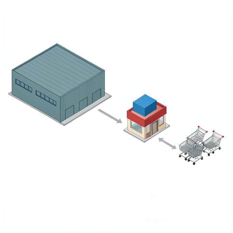
Two-Echelon Supply Chain Structure
AI-generated conceptual illustration (a warehouse and a retail store). It explains the idea and does not show study data.
View source evidence ↗Figures & tables
From the original paper Table 1
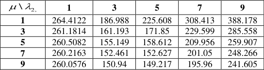 Table 3
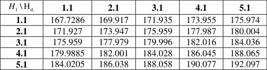 Table 4
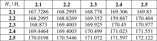 Table 5
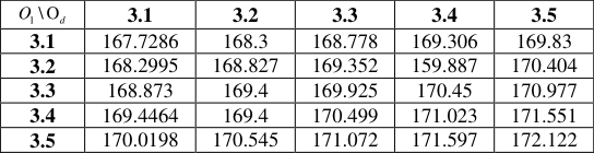 Table 6
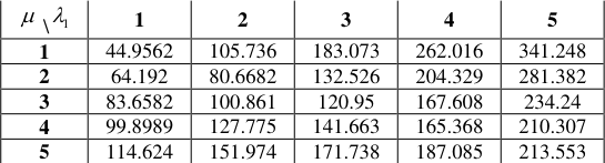 Table 2
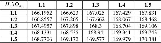 Table 7
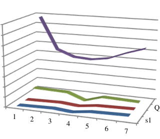 Figure 1
Introduction
This paper investigates the substitutable product inventory control systems in supply chain. When different products are sold by a retailer, substitution between these products causes the retailers to manage their order quantities in a competitive environment. In this article, we examine the nature of continuous review inventory control system facing stochastic independent demand in supply chain. Substitutable product inventory problem was first studied by McGillivray and Silver [1] in the Economic Order Quantity (EOQ) context. Later, Parlar and Goyal [19] and Khouja and Mehrez and Rabinowitz [18] gave single-period formulations for an inventory system with two substitutable products independently of each other. In [21] , Parlar proposed a Markov Decision Process model to find the optimal ordering policies for perishable and substitutable products from the point of view of one retailer. Parlar's study in [25] is a game theoretic analysis of the inventory control under substitutable demand. He modeled the two-product single period problem as a two-person nonzero-sum game and showed that there exists a unique Nash equilibrium. Study on multi-echelon systems are much less compared to those on single commodity systems. The determination of optimal policies and the problems related to a multi-echelon systems are, to some extent, dealt by Veinott and Wagner [30] and Veinott [31] . Sivazlian [28] discussed the stationary characteristics of a multi commodity single period inventory system.The terms multi-echelon or multi-level production distribution network and also synonymous with such networks (supply chain) when on items move through more than one steps before reaching the final customer. Inventory exist throughout the supply chain in various form for various reasons. At any manufacturing point they may exist as rawmaterials, work-in process or finished goods. The main objective for a multi-echelon inventory model is to coordinate the inventories at the various echelons so as to minimize the total cost associated with the entire multi-echelon inventory system. This is a natural objective for a fully integrated corporation that operates the entire system. It might also be a suitable objective when certain echelons are managed by either the suppliers or the retailers of the company. Multi-echelon inventory system has been studied by many researchers and its applications in supply chain management has proved worthy in recent literature. As supply chains integrates many operators in the network and optimize the total cost involved without compromising as customer service efficiency. The first quantitative analysis in inventory studies Started with the work of Harris [13] . Clark and Scarf [8] had put forward the multi-echelon inventory first. They analyzed a N-echelon pipelining system without considering a lot size. One of the oldest papers in the field of continuous review multi-echelon inventory system is written by Sherbrooke in 1968.Hadley, G and Whitin, T. M., [12] , Naddor. E [24] analyses various inventory Systems. HP's (Hawlett Packard) Strategic Planning and Modeling (SPaM) group initiated this kind of research in 1977. Sivazlian and Stanfel [27] analyzed a two commodity single period inventory system. Kalpakam and Arivarignan [15] analyzed a multi-item inventory model with renewal demands under a joint replenishment policy. They assumed instantaneous supply of items and obtain various operational characteristics and also an expression for the long run total expected cost rate. Krishnamoorthy et al., [16] analyzed a two commodity continuous review inventory system with zero lead time. A two commodity problem with Markov shift in demand for the type of commodity required, is considered by Krishnamoorthy and Varghese [17] . They obtain a characterization for limiting probability distribution to be uniform. Associated optimization problems were discussed in all these cases. However in all these cases zero lead time is assumed. A Complete review on multi echelon inventory model was provided by Benito M. Beamon [6] . Sven Axsater [5] proposed an approximate model of inventory structure in SC. He assumed (S-1, S) polices in the Deport-Base systems for repairable items in the American Air Force and could approximate the average inventory and stock out level in bases. Anbazhagan and Arivarignan [2,3] have analyzed two commodity inventory system undervarious ordering policies. Yadavalli et al., [32] have analyzed a model with joint ordering policy and varying order quantities. Yadavalli et al., [33] have considered a two commodity substitutable inventory system with Poisson demands and arbitrarily distributed lead time. In a very recent paper, Anbazhagan et al. [4] considered analysis of two commodity inventory system withcompliment for bulk demand in which, one of the items for the major item, with random lead time but instantaneous replenishment for the gift item are considered. The lost sales for major item is also assumed when the items are out of stock. The above model is studied only at single location( Lower echelon). We extend the same in to multi-echelon structure (Supply Chain). The rest of the paper is organized as follows. The model formulation is described in section 2, along with some important notations used in the paper. In section 3, steady state analysis are done: Section 4 deals with the derivation of operating characteristics of the system. In section 5, the cost analysis for the operation. Section 6 provides Numerical examples and sensitivity analysis.
Model 2.1 The Problem Description
The inventory control system considered in this paper is defined as follows. Tow Substitutable finished products (A & B) are supplied from manufacturer to supplier which adopts (0,M) replenishment policy then the product is supplied to retailer who adopts (s i , S i ) policy. The demand at retailer node follows an independent Poisson distribution with rate 𝜆 1 for one product A and 𝜆 2 for product B. When the inventory of one of the product reaches zero the demand for the product is substitutable with the other product with probability p and similar argument for another product with probability q so that p +q =1. The demands that occur when both the products are out of stock are partially backlogged. The replacement of item in terms of product is made from supplier to retailer is administrated with exponential distribution having parameter 0.
The maximum inventory level at retailer node for product A and B are Si, and the recorder point is si and the ordering quantity is Q(=S i -s i ) items. The maximum inventory at supplier is M(=nQ).
Analysis
Let 1(𝑡)and 𝐼 2 (𝑡) denote the on hand Inventory levels of product A and B respectively at retailer and 𝐼 𝑑 (𝑡)denote the on hand inventory level of both products at supplier at time t+. We define I (t) = {(𝐼 1 (𝑡), 𝐼 2 (𝑡), 𝐼 𝑑 (𝑡)): t ≥ 0 }as Markov process with state space E = { ( i, j,k) | i = S 1 ,S 1 -1 .....0,-1,-2,…-b j = S 2 ,S 2 -1 .....0,-1,-2,…-b, k=Q,2Q,.....nQ }. Since E is finite and all its states are aperiodic, recurrent, non-null and also irreducible. That is all the states are Ergodic. Hence the limiting distribution exists and is independent of the initial state. The infinitesimal generator matrix of this process C = ( a ( i, j,
can be obtained from the following arguments. The arrival of a demand for product A at retailer make a state transition in the Markov process from (i, j, k) to ( i-1, j, k ) with the intensity of transition ( 1 >0).i=1,2,….S 1
The arrival of a demand for product B at retailer make a state transition in the Markov process from (i, j, k) to ( i, j-1, k) with the intensity of transition ( 2 >0).j= 1,2……S 2 The arrival of common direct demand for product A and B distinct for make a transits in the Markov process from (i, j, k) to (i, j, k-Q) with the indirect of transition d When the inventory level of product A is zero, then the the arrival of a demand for product A at retailer make a state transition in the Markov process from (i, j, k) to ( i, j-1, k )
with the intensity of transition
The sub matrices A and B are given by
b [M]
q p p S ,S 1.....0, 1,... b 0 otherwise
Steady State Analysis
The structure of the infinitesimal matrix C, reveals that the state space E of the Markov process { I (t): t ≥ 0 } is finite and irreducible. Let the limiting probability distribution of the inventory level process be
the steady state probability that the system be in state (i, j, k). By solving the above system of equations, together with normalizing condition ( , , ) ,
, the steady probability of all the system states are obtained.
Operating characteristic
In this section we derive some important system performance measures.
Average inventory Level
The event I 1 , I 2 denote the average inventory level for products A and B respectively at retailer node and I d denote the average inventory level at distributor node
Mean Reorder Rate
Let R 1 , R 2 , denote the mean reorder rate for products A and B, retailer and R d denote the mean reorder rate for products at distributor respectively, (
Shortage rate
Shortage occur at retailer only for main product. LetS r be the shortage rate at retailer for main product, then
S ( )
S ( )
Cost analysis
In this section we impose a cost structure for the proposed model and analyze it by the criteria of minimization of long run total expected cost per unit time. The long run expected cost rate TC(s 1 , s 2 , Qis given by
Although we have not proved analytically the convexity of the cost function TC(s 1 , s 2 , Qour experience with considerable number of numerical examples indicate that TC(s 1 , s 2 , Q) for fixed 'S 1 and S 2 ' appears to be convex ins. In some cases it turned out to be increasing function of s. For large number case of TC(s 1 , s 2 , Q) revealed a locally convex structure. Hence we adopted the numerical search procedure to determine the optimal value of 's'
Numerical Example and Sensitivity Analysis 6.1 Numerical Example
In this section we discuss the problem of minimizing the structure. We assume H 2 ≤ H 1 ≤ H d, i.e, the holding cost for product B at retailer node is less than that of product A and the holding cost of both products is less than that of products at distributor node. Also O 2 ≤ O 1 ≤O d the ordering cost at retailer node for product B is less than that of product A. Also the ordering cost at the distributor is greater than that of both products at retailer node.
The results we obtained in the steady state case may be illustrated through the following numerical example,
The cost for different reorder level are given by For the inventory capacity S 1 and S 2 , the optimal reorder level s 1 , and s 2 and optimal cost TC(s 1 , s 2 , Q)are indicated by the symbol *. The Convexity of the cost function is given in the graph with common reorder point s (both s 1 , and s 2 ).
Sensitivity Analysis
Below tables are represented a numerical study to exhibit the sensitivity of the system on the effect of varying different parameters.
For the following cost structureS 1 =16, S 2 =16 M = 80, It is observed that from the table, the total expect cost TC(s 1 , s 2 , Q)is increases with the cost increases.
Conclusion
This paper deals with a two echelon Inventory system with two substitutable products A and B.. The structure of the chain allows vertical Movements of goods. It would be calculating to analyze the problem with general distribution. The author is working in their directions and further results will be reported soon.
Figures and tables from the paper
| s1 | 1 | 2 | 3 | 4* | 5 | 6 | 7 |
|---|---|---|---|---|---|---|---|
| s2 | 1 | 2 | 3 | 4* | 5 | 6 | 7 |
| Q | 15 | 14 | 13 | 12* | 11 | 10 | 9 |
| TC(s1, s2, Q) | 155.835611 | 90.63277 | 77.55012 | 75.28077 | 80.75253 | 94.54283 | 105.9115 |
Table text extracted from the original PDF; superscript letters are shown inline. The original table image is below.
View original table image
| \ 2, | 1 | 3 | 5 | 7 | 9 |
|---|---|---|---|---|---|
| 1 | 264.4122 | 186.988 | 225.608 | 308.413 | 388.178 |
| 3 | 261.1814 | 161.193 | 171.85 | 229.599 | 285.558 |
| 5 | 260.5082 | 155.149 | 158.612 | 209.956 | 259.907 |
| 7 | 260.2163 | 152.461 | 152.627 | 201.05 | 248.266 |
| 9 | 260.0576 | 150.94 | 149.217 | 195.96 | 241.605 |
Table text extracted from the original PDF; superscript letters are shown inline. The original table image is below.
View original table image
| H \ H 1 d, | 1.1 | 2.1 | 3.1 | 4.1 | 5.1 |
|---|---|---|---|---|---|
| 1.1 | 167.7286 | 169.917 | 171.935 | 173.955 | 175.974 |
| 2.1 | 171.927 | 173.947 | 175.959 | 177.987 | 180.004 |
| 3.1 | 175.959 | 177.979 | 179.996 | 182.016 | 184.036 |
| 4.1 | 179.9885 | 182.001 | 184.028 | 186.045 | 188.065 |
| 5.1 | 184.0205 | 186.038 | 188.058 | 190.077 | 192.097 |
Table text extracted from the original PDF; superscript letters are shown inline. The original table image is below.
View original table image
| H \ H 2 1 | 2.1 | 2.2 | 2.3 | 2.4 | 2.5 |
|---|---|---|---|---|---|
| 2.1 | 167.7286 | 168.2995 | 168.778 | 169.306 | 169.83 |
| 2.2 | 168.2995 | 168.8269 | 169.352 | 159.887 | 170.404 |
| 2.3 | 168.873 | 169.4003 | 169.925 | 170.45 | 170.977 |
| 2.4 | 169.4464 | 169.4003 | 170.499 | 171.023 | 171.551 |
| 2.5 | 170.0198 | 170.5446 | 171.072 | 171.597 | 172.122 |
Table text extracted from the original PDF; superscript letters are shown inline. The original table image is below.
View original table image
| O \ O 1 d | 3.1 | 3.2 | 3.3 | 3.4 | 3.5 |
|---|---|---|---|---|---|
| 3.1 | 167.7286 | 168.3 | 168.778 | 169.306 | 169.83 |
| 3.2 | 168.2995 | 168.827 | 169.352 | 159.887 | 170.404 |
| 3.3 | 168.873 | 169.4 | 169.925 | 170.45 | 170.977 |
| 3.4 | 169.4464 | 169.4 | 170.499 | 171.023 | 171.551 |
| 3.5 | 170.0198 | 170.545 | 171.072 | 171.597 | 172.122 |
Table text extracted from the original PDF; superscript letters are shown inline. The original table image is below.
View original table image
| \ 1 | 1 | 2 | 3 | 4 | 5 |
|---|---|---|---|---|---|
| 1 | 44.9562 | 105.736 | 183.073 | 262.016 | 341.248 |
| 2 | 64.192 | 80.6682 | 132.526 | 204.329 | 281.382 |
| 3 | 83.6582 | 100.861 | 120.95 | 167.608 | 234.24 |
| 4 | 99.8989 | 127.775 | 141.663 | 165.368 | 210.307 |
| 5 | 114.624 | 151.974 | 171.738 | 187.085 | 213.553 |
Table text extracted from the original PDF; superscript letters are shown inline. The original table image is below.
View original table image
| H \ O 1 d; | 1.1 | 1.2 | 1.3 | 1.4 | 1.5 |
|---|---|---|---|---|---|
| 1.1 | 166.1952 | 166.623 | 167.025 | 167.429 | 167.831 |
| 1.2 | 166.8557 | 167.265 | 167.662 | 168.067 | 168.468 |
| 1.3 | 167.4957 | 167.898 | 168.3 | 168.704 | 169.106 |
| 1.4 | 168.1331 | 168.535 | 168.94 | 169.341 | 169.743 |
| 1.5 | 168.7706 | 169.172 | 169.577 | 169.979 | 170.381 |
Table text extracted from the original PDF; superscript letters are shown inline. The original table image is below.
View original table image
References
33 in the original paper- McGillivray AR, Silver EA. Some Concepts for Inventory Control under Substitutable Demand. Infor, 1978; 16:47-63.
- Anbazhagan N, Arivarignan G. Analysis of twocommodity Markovian inventory system with lead time. The Korean Journal of Computational and Applied Mathematics. 2001; 8(2):427-438.
- Anbazhagan N, Arivarignan G. Two-commodity continuous review inventory system with Coordinated reorder policy. International Journal of Information and Management Sciences. 2000; 11(3):19-30.
- Anbazhagan N, Jeganathan K. Two-Commodity Markovian Inventory System with Compliment and Retrial Demand: British Journal of Mathematics & Computer Science. 2013; 3(2):115-134.
- Axsater S. Exact and approximate evaluation of batch ordering policies for two level inventory systems. Oper. Res. 1993; 41:777-785.
- Benita M Beamon. Supply Chain Design and Analysis: Models and Methods. International Journal of Production Economics. 1998; 55(3):281-294.
- Cinlar E. Introduction to Stochastic 'Processes, Prentice Hall, Engle-wood Cliffs, NJ, 1975.
- Clark AJ, Scarf H. Optimal Policies for a Multi-Echelon Inventory Problem. Management Science, 1960; 6(4):475-490.
- Iglehart DL. The Optimality of (s,S) Policies in the Infinite Horizon Dynamic Inventory Problem. Management Science, 1963; 9:259-267.
- Ignall E, Veinott AF. Optimality of Myopic Inventory Policies for Several Substitute Products. Management Science, 1969; 15:284-304.
- Scarf H. The Optimality of (s,S) policies in the Dynamic Inventory Problem. Mathematical Methods in the Social Sciences, 1960, 196-202.
- Hadley G, Whitin TM. Analysis of inventory systems, Prentice-Hall, Englewood Cliff, 1963.
- Harris F. Operations and costs, Factory management series, A.W. Shah Co., Chicago, 1915, 48-52.
- Filar JA, Schultz TA, Thuijsman F, Vrieze DJ. Nonlinear Programming and Stationary Equilibria in Stochastic Games. Mathematical Programming, 1991; 50:227-238.
- Kalpakam S, Arivarigan G. A coordinated multicommodity (s, S) inventory system. Mathematical and Computer Modelling. 1993; 18:69-73.
- Krishnamoorthy A, IqbalBasha R, Lakshmy B. Analysis of a two commodity problem. International Journal of Information and Management Sciences. 1994; 5(1):127136.
- Krishnamoorthy A, Varghese TV. A two commodity inventory problem. International Journal of Information and Management Sciences. 1994; 5(3):55-70.
- Khouja M, Mehrez A, Rabinowitz G. A Two-Item Newsboy Problem with Substitutability. International Journal of Production Economics. 1996; 44:267-275.
- Parlar M, Goyal SK. Optimal Ordering Decisions for Two Substitutable Products with Stochastic Demands. Opsearch, 1984; 21:1-15.
- Parlar M. Game Theoretic Analysis of the Substitutable Product Inventory Problem with Random Demands. Naval Research Logistics, 1988; 35:397-409.
- Parlar M. Optimal Ordering Policies for A Perishable and Substitutable Product: A Markov Decision Model. Infor, 1985; 23:182-195.
- Sobel MJ. Myopic Solutions of Markov Decision Processes and Stochastic Games. Operations Research, 1981; 29:995-1009.
- Medhi J. Stochastic processes, Third edition, New Age International Publishers, New Delhi, 2009.
- Naddor E. Inventory System, John Wiley and Sons, New York, 1966. Ordering policies. International Journal of Management and Systems. 2003; 19(2):129-144.
- Wang Q, Parlar M. A Three-Person Game Theory Model arising in Stochastic Inventory Control Theory. European Journal of Operations Research. 1994; 76:83-97.
- Bellman R, Glicksberg I, Gross O. On the Optimal Inventory Equation. Management Science. 1955; 2:83104.
- Sivazlian BD, Stanfel LE. Analysis of systems in Operations Research. First edition. Prentice Hall, 1974.
- Sivazlian BD. Stationary analysis of a multicommodity inventory system with interacting set-up costs. SIAM Journal of Applied Mathematics. 1975; 20(2):264-278.
- Raghavan TES, Filar JA. Algorithms for Stochastic Games-A Survey. ZOR-Methods and Models of Operations Research, 1991; 35:437-472.
- Veinott AF, Wagner HM. Computing optimal (s, S) inventory policies. Management Science. 1965; 11:525552.
- Veinott AF. The status of mathematical inventory theory. Management Science 1966; 12:745-777.
- Yadavalli VSS, Anbazhagan N, Arivarignan G. A two commodity continuous review inventory system with lost sales. Stochastic Analysis and Applications. 2004; 22:479-497.
- Yadavalli VSS, De WC, Udayabaskaran S. A substitutable two-product inventory system with joint ordering policy and common demand. Applied Mathematics and Computation. 2006; 172(2):1257-1271.