
Research article · 2020 · Full text
International Journal of Statistics and Applied MathematicsResearch on the mutual influence between the population of deer and grass quantity based on difference method
Volume 5(4) · Pages 49–55
Research areasMathematical and Theoretical Epidemiology and Ecology ModelsEcology and biodiversity studiesAnimal Diversity and Health Studies
Abstract
Author-writtenBy establishing different difference equation models, this paper analyzes the relationship between the population of deer and grass quantity in the food chain in detailed. It is found that when the maximum quantity of grass changes the trend of the population of the two species is likely to be different: when the maximum quantity of grass is small, the grass quantity will decrease first and then increase, and when the grass quantity is large, it will increase first and then decrease. The trend of the deer population is opposite to the trend of the grass quantity.
Summary
Source-checkedPlain-language reading of the full paper, prepared with AI and checked against the text. Each point links to the authors' own words.
Why it matters
- Interactions between adjacent species in food chains, where one creature feeds on another, significantly impact the survival and development of those biological populations. View evidence ↗
- While difference equations have been used to analyze species interactions, previous applications are generally considered not comprehensive enough. View evidence ↗
The question
- The study aims to analyze the population trends of deer and grass under various initial quantities and environmental conditions to provide more comprehensive results. View evidence ↗
What they did
- The model assumes a Prey-Predator relationship where grass growth follows a discrete logistic law and populations are only affected by each other, ignoring external factors. View evidence ↗
- The mathematical model utilizes parameters for grass growth rate (r), maximum grass quantity (N), deer consumption (a), deer mortality (b), and deer compensation rate (d). View evidence ↗
- MATLAB software was used to simulate and visualize the population changes of deer and grass. View evidence ↗
What they found
- Under the specified parameters, the populations eventually stabilize at approximately 1800 for grass and 600 for deer. View evidence ↗
- The initial trend of grass quantity depends on its maximum capacity: it decreases then increases when the maximum is 1000, but increases then decreases when the maximum is 5000. View evidence ↗
- Changing deer consumption affects the stable deer population: a consumption rate of 1 leads to 960 deer, while a rate of 2 reduces the stable deer population to 500, though grass remains stable at 1800. View evidence ↗
- Higher deer mortality rates shorten the fluctuation period; a rate of 0.7 results in 100 years of fluctuation, whereas a rate of 0.95 reduces this to about 40 years. View evidence ↗
What it means
- The authors conclude that humans can manage species populations by controlling initial quantities, grass growth, and deer birth and death rates. View evidence ↗
Visual summary
1 visualsIllustrations explain the paper; they do not show study data.
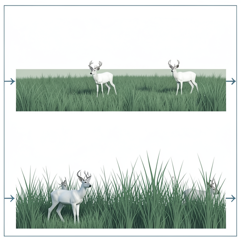
Impact of Maximum Grass Quantity on Initial Trends
AI-generated conceptual illustration (white-tailed deer and green pasture grass). It explains the idea and does not show study data.
View source evidence ↗Figures & tables
From the original paper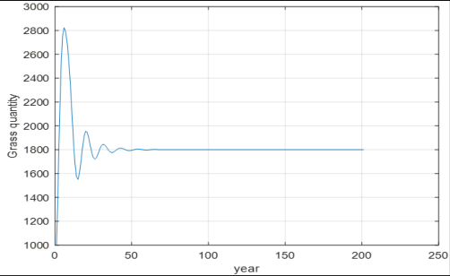 Figure 1
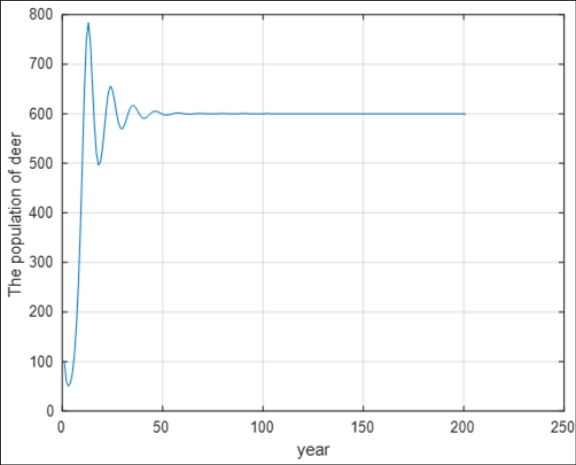 Figure 2
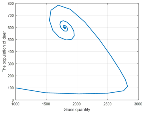 Figure 3
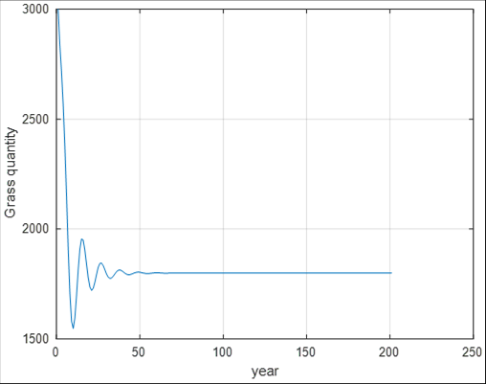 Figure 4
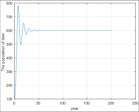 Figure 5
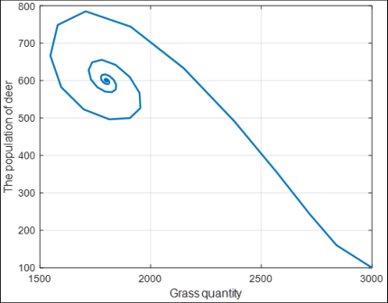 Figure 6
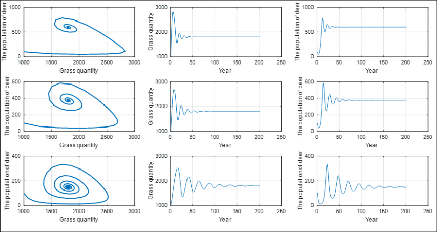 Figure 7
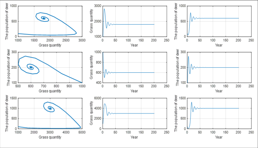 Figure 8
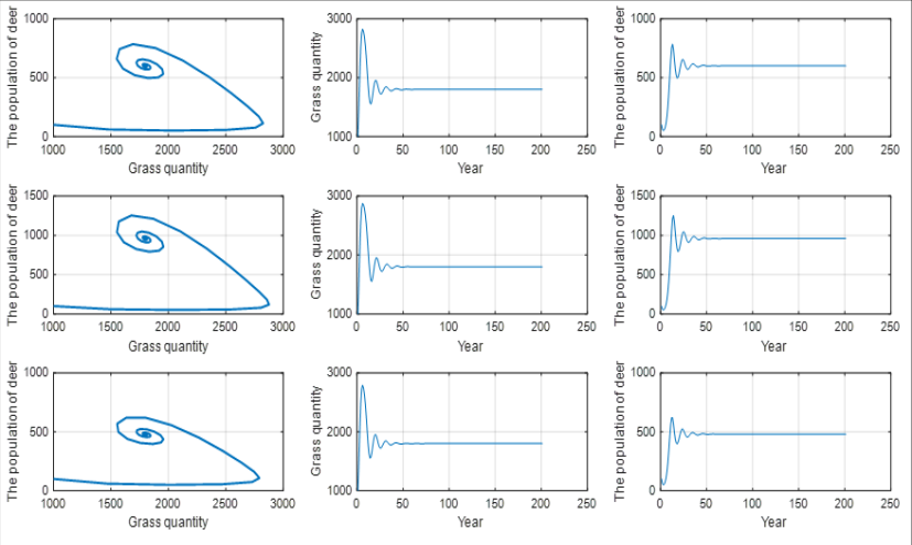 Figure 9
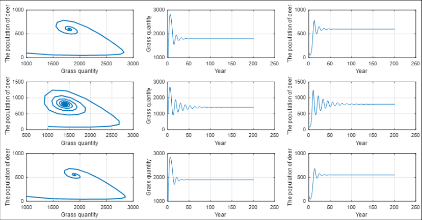 Figure 10
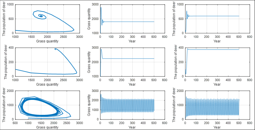 Figure 11
Introduction
A creature in nature often feeds on another one, and at the same time it provides for one or more other species as food, which forms food chains in the ecosystem [1,2] . The interaction between two adjacent species in a food chain has greatly affected the survival and development of this two biological populations [3][4][5][6][7][8] . In this case, the method of difference equation has been applied to analyze this problem, but generally speaking, it is not comprehensive enough [9][10][11][12][13] . Based on previous studies, this paper takes two common species in the ecosystem-deer and grass as an example to analyze the trend of two populations with different initial quantities and in different environmental conditions to push the research in this field further and get more valuable results.
The difference equation model of the population of two species 2.1 The difference equation of the population of two species
Firstly, according to the ecological knowledge [1][2][3][4] , the basic assumptions are made as follows:
1. The population of deer and grass quantity are only affected by grass or deer themselves, and other external factors are not considered; 2. The growth of grass follows the law of discrete form logistic; 3. Grass is the prey and deer is the predator, so they follow the Prey-Predator model. Now supposing that r represents the annual intrinsic growth rate of grass, N represents the maximum quantity of grass, a represents the quantity of the deer's annual consumption of grass, b represents the annual mortality of the deer herd, d represents the deer's annual compensation rate, 𝑥 𝑘 represents the grass quantity in the kth year , and 𝑦 𝑘 represents the population of deer in the kth year, then according to the hypothesis, the relationship between the grass quantity and the population of deer obeys the following difference equations [5][6][7][8][9][10][11][12] :
The initial value is ) , ( 0 0 y x .
The calculation of the equilibrium point and its stability judgment
in equation (1) solve the equilibrium point, and we get the point:
The stability of this equilibrium point will be analyzed below.
The equivalent form of difference equations ( 1) is as follows:
Therefore, the difference equations (3) are discrete forms of differential equations (4):
It can be verified that the equilibrium point (2) of the difference equation ( 1) is also the equilibrium point of the differential equations ( 4), which means that the stability of the equilibrium point (2) is the same in two groups of equations. Therefore, we will analyze the stability of the equilibrium point (2) of the difference equations ( 1) according the differential equations ( 4). According to the relevant knowledge of the stability theory of differential equations, the Jacobian matrix of the differential equations (4) at the equilibrium point ( 2) is calculated as: 3. The cases that the initial values of the population of two species are changed 3.1 Equilibrium point and its stability of the population of two species Now we consider two cases that the initial values of the population of deer and grass quantity take two different values under a fixed environmental condition. The first case is that the initial population of deer is 100 and the initial quantity of grass is 1000; the second case is that the initial population of deer is 100 and the initial grass quantity is 3000. We suppose that the annual intrinsic growth rate of grass is 0.8, and the maximum quantity of grass is 3000. When the grass is flourishing, each deer consumes 1.6 quantity of grass annually. Without grass, the annual mortality of deer is as high as 0.9 percent. The existence of grass can compensate 1.5 deer for deer's death when the grass quantity is the most. According to formula (2) (7), the equilibrium points of the number of two populations are same when the above initial values are different. We suppose that According to the analysis of the stability of the equilibrium point above, it can be found that this equilibrium point is a stable focus. And when time tends to infinity, the grass quantity gradually stabilizes at about 1800, and the population of deer gradually stabilizes at about 600. However, the change trend of the number of two populations is still unclear. Therefore, in order to make the change process of two populations more detailed, two cases of different initial values are discussed and explained in the next.
The case that the initial grass quantity is 1000 and the initial population of deer is 100
When the initial value is It can be seen from Figure 1 that the grass quantity increases in the initial period of time. The grass quantity reaches its maximum 2824.5, then decreases sharply, and then increases again. After repeating this process, it will be stable at about 1800 after about 50 years. It can be seen from Figure 2, the population of deer decreases slightly in the initial period of time, and then increases continuously. The maximum population of deer reaches 655, then decreases again, and then rises again. After repeating this process, it will be stable at about 600 after about 50 years.
It can be seen from Figure 3 that the increase of the grass quantity can promote the the population of deer to increase, while the increase of the population of deer will inhibit the grass quantity from increasing. The interaction between the two species makes the population of two species adjust with fluctuation, and finally stabilize at the equilibrium point ) 600 , 1800 ( ) , ( = q p after 50 years.
The case that the initial grass quantity is 3000 and the initial population of deer is 100
When the initial value is, ) 100 , 1000 ( ) , (
we use MATLAB to draw the images the populations of two species again, as shown in Figures 4, 5 and6. It can be seen from Figure 4 that the grass quantity decreases in the initial period of time. The grass quantity reaches its minimum 1792, then increases again, and then decreases again. After repeating this process, it will be stable at about 1800 after about 50 years.
It can be seen from Figure 5 that the population of deer increases greatly in the initial period of time. The maximum number reaches 785, then decreases, and then rises again. After repeating this process, and it is stable at about 600 in about 50 years. It can be seen from Figure 6 that the grass quantity is high at the beginning, which makes the population of deer increases greatly. However, because the number of deer is too large, the grass quantity decreases sharply, making the population of deer decreases next. The between the two species makes the population of two species change with fluctuation, and they finally stabilize at the equilibrium point ) 600 , 1800 ( ) , ( = q p after about 50 years. Comparing the above two cases, the different condition is different initial grass quantity. When the grass quantity is higher, the grass quantity first decreases and then increases, and the population of deer first increases and then decreases; when the grass quantity is small, the grass quantity first increases and then decreases, and the population of deer first decreases and then increases. In both cases, the population of two species tends towards the point ) 600 , 1800 ( at last. , and the number of fluctuations is also more. Therefore, this equilibrium point looks like a center point
Conclusion
Different values of the above parameters represent different initial values of the population of species and different environmental conditions. Therefore, the following laws can be obtained through the above analysis: 1. Under the same environmental conditions, if the initial values of the grass quantity and the population of deer take different sets of values, the final stability of the population of the two species is the same, and if both are stable, then their stable points can be calculated the same; 2. When the intrinsic growth rate of grass is large, the fluctuation time of the grass quantity and the population of deer is shorter and the fluctuation range is smaller. While the intrinsic growth rate of grass is small, the fluctuation time is longer and the fluctuation range is larger; 3. Both the trends of the grass quantity and the population of deer may change when the maximum quantity of grass changes. When the maximum grass quantity is small, the grass quantity will first decrease and then increase. While the maximum quantity of grass is large, grass quantity will first increase and then decrease. Correspondingly, the trend of the population of deer is opposite to the trend of grass quantity; 4. When the annual mortality rate of deer is large, the fluctuation time of the grass quantity and the population of deer is short, while the death rate of the deer is small, the fluctuation time is long;
5. When the annual compensation rate of deer is large, the fluctuation time of the grass quantity and the population of deer is long, while the annual compensation rate of deer is small, the fluctuation time is short.
In conclusion, to achieve the desired effect of the population of these two species, humans can control the initial population of and deer and grass quantity, the growth of grass, and the death and birth of deer etc.
Figures and tables from the paper
References
20 in the original paper- Jiang ZH. Integrated ecosystem management. Beijing: China Forestry Press, 2006.
- Walcott KA. Ecosystem. Beijing: Science Press, 2002.
- Wang GQ, Tian Y. On grassland ecosystem and grassland ecological culture. Frontier. 2013; (03):162166.
- En H. Relationship between the change of grassland ecological material cycle and grassland degradation and restoration measures. Environment and development. 2017; 29(05):207-209, 211.
- Wu YW. Study on single population optimal capture strategy model with age structure. Chongqing University, 2006.
- Lin YH. Study on dynamic behavior of four two species model. Fuzhou University, 2014.
- Li XK. Stability and numerical simulation of two species competitive system. Journal of Three Gorges University. 2012; 34(04):101-103.
- Dai YX. Two results on the recovery rate of two species predator-prey system. Liaoning University of engineering and technology, 2011.
- Ma XM and Liu H, Ma G & Ma M. Computer simulation of discrete two species competition ecological mathematical model. Journal of Gansu Union University. 2010; 24 (05):44-46.
- Chen Z and Gao Y. Harvesting model and control of two species predator prey system. Journal of Biomathematics. 2009; 24(03):419-426.
- Wu CG. A predator-prey population dynamics model and numerical simulation. Central University for nationalities, 2009.
- Li DL. Study on two species predator-prey system in ecosystem. Northeast Normal University, 2007.
- Zhang SY and Lu GQ. Some examples of whole system model of grassland ecosystem and the function of the model. Foreign animal husbandry. Grassland and pasture. 1983; (03):1-5.
- Wang GX. Ordinary differential equations. Beijing: Higher Education Press, 2006.
- Yan GZ. Ordinary differential equation. Beijing: Science Press, 2012.
- Walter W. Ordinary differential equations. New York: Springer-Verlag, 2003.
- Cao WD, Yi SH, Wang YL. Prediction model of population change of plateau pika. Journal of Southwest University. 2019; 45(02):125-133.
- Li CC. Population structure and dynamics of Yegu grass and Leymus chinensis in mixed community of Songnen grassland. Northeast Normal University, 2014.
- Bu ZJ. Population ecology of several plants in the poor nutrient peat swamp of Northeast China. Northeast Normal University, 2004.
- Zou YD, Ma F, Meng QL, Hu LJ, Huang SX. Population dynamics of two wheat aphids at different growth stages. Journal of Biomathematics. 1994; (03):78-83.