
Research article · 2020 · Full text
International Journal of Statistics and Applied MathematicsOn a statistical control of a technological process described by a two-dimensional normal distribution
Volume 5(4) · Pages 131–134 · DOI: 10.22271/maths.2020.v5.i4b.561 ↗
Research areasStatistical and Computational Modeling
Abstract
Author-writtenIn the papera methodology for controlling a technological process described by a two-dimensional normal distribution using new control charts is given, where the control value is Kolmogorov's statistics ρx and ρy and a correlation coefficient (rxy). Using these control charts shows the control of the machine producing the shotgun shells (weapons or other shotgun shells). Control charts are based on Kolmogorov’s consentcriterion and Fisher’s criterion of linear dependence of the components of a random normal vector.
Summary
Source-checkedPlain-language reading of the full paper, prepared with AI and checked against the text. Each point links to the authors' own words.
Why it matters
- Mathematical statistics are used to develop quality management systems that actively prevent defects during manufacturing. View evidence ↗
- The study uses the manufacturing of shotgun shells with a nominal bore diameter of 30mm as a practical example for process control. View evidence ↗
- Process control for these shells involves measuring deviations from the nominal diameter in two mutually perpendicular planes, represented as variables X and Y. View evidence ↗
The question
- The paper aims to provide a methodology for controlling a technological process described by a two-dimensional normal distribution using new control charts based on Kolmogorov's statistics and a correlation coefficient. View evidence ↗
What they did
- The researchers constructed ρx and ρy control charts based on the Kolmogorov consent criterion to verify the normality of the X and Y data sets. View evidence ↗
- A ρxy control chart based on the Fisher criterion was used to check the linear dependence between the X and Y variables. View evidence ↗
- To establish baseline parameters, a sample of 150 measurements was taken from a standard, perfectly working machine. View evidence ↗
- For a sample size of 150 and a significance level of α = 0.05, the upper control limit (UCL) for the ρ charts was calculated as 0.07. View evidence ↗
- The control limits for the ρxy chart were determined to be an upper limit (UCL) of 1 and a lower limit (LCL) of 0.39. View evidence ↗
What they found
- The power function G(rxy) showed high percentages at moments j=4 (96%), j=6 (99%), and j=7 (91%), indicating a need to stop the machine. View evidence ↗
What it means
- The authors conclude that the process was in a statistically controlled state at moments j= 1, 2, 3, 5, and 8. View evidence ↗
- For moments where the process left the controlled state, the authors recommend collaborating with specialists to identify the causes. View evidence ↗
Visual summary
1 visualsIllustrations explain the paper; they do not show study data.

Control Chart Framework
AI-generated conceptual illustration (Industrial precision machining components). It explains the idea and does not show study data.
View source evidence ↗Figures & tables
From the original paper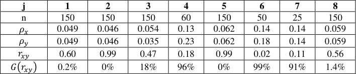 Table 1
Introduction
The need for active methods of preventing defects in the manufacturing process has led to the development of methods and quality management systems based on methods of mathematical statistics. In this case, one of the most important problems is the control of the machine. In the paper,as an example, we will consider one of such machines manufacturing parts and show the statistical control of this process. Let the shotgun shells (weapon shells, cylinder shells, etc.) with bore nominal diameter 𝑑 = 30𝑚𝑚 be manufactured on a central lathe. The control of the bore diameter of the shotgun shells is carried out in two mutually perpendicular planes. Deviations from the nominal in these planes are denoted by 𝑋 and 𝑌. In [1] it was proved that these random variables are distributed normally with defined parameters and are linearly dependent. Machine control described by a two-dimensional random vector(𝑋, 𝑌):
In practice, these five parameters are taken as technical standards. Here 𝜇 𝑜𝑥 , 𝜇 𝑜𝑦 are mathematical expectations and 𝜎 𝑜𝑥 2 , 𝜎 𝑜𝑦 2 are variances of 𝑋 and 𝑌 respectively, 𝜌 𝑥𝑦 𝑜 is the correlation coefficient of X and Y. If at certain moments 𝑗 = 1, 2, … , 𝑡 we take a sample (or instantaneous sample) from (𝑋, 𝑌) with volume n:
(𝑋 𝑗 , 𝑌 𝑗 ) = {(𝑥 𝑗1, 𝑦 𝑗1 ); (𝑥 𝑗2 , 𝑦 𝑗2 ), … , (𝑥 𝑗𝑛 , 𝑦 𝑗𝑛 )}, evaluating the five parameters, we check the shape of the two-dimensional density concerning a given standard, and if one observes that the shape is almost preserved, then we say that the process is in a statistically controlled state. Note that deviations from the standard, can probably due to random reasons acting on the machine. Otherwise, we say that the process exits a statistically controlled state and is unpredictable, because of non-random factors which is affecting to the machine. Mathematical verification of the above leads to the verification of statistical hypotheses Using the conditional densities 𝑓( 𝑦 𝑥 ⁄ ) and 𝑓( 𝑥 𝑦 ⁄ ) [2] one may prove that 𝑋 and 𝑌 are linearly dependent, i.e. C is valid, where 𝑓 is the density function of the Gaussian distribution). The inverse problem: "From A, B and C it follows D" is not always solvable. But our (𝑋, 𝑌) is distributed normally, therefore 𝑋 and 𝑌 are linearly dependent and D is valid. In practice, using of control charts (CC) is convenient and visual (see, for example, [3] ) instead of testing hypotheses. Therefore, here we use the CC obtained in [4] and [5] to solve problems A, B and C. Further, we will give the basic rules arising from the proved theorems in [4] and [5] .
Materials and Methods
The main characteristics of CC are LCL (lower control limit), UCL (upper control limit), CL (central line) and control value 𝐾 𝑗 = 𝐾(𝑋 𝑗 , 𝑌 𝑗 ), 𝑗 = 1, 2, … , 𝑡. It is known that accuracy of CC are carried out through power functions and LCL and UCL can be found if one knows the distribution of the control value. In [4] a CC was obtained using the Kolmogorov'sconsent criterion to verify the normality of the general set. Using these results, we construct 𝜌 𝑥 and 𝜌 𝑦 charts here to verify the normality of the sets 𝑋 and 𝑌. In [5] , based on the Fisher criterion, the characteristics of the 𝜌 𝑥𝑦 chart was obtained, which checks the linear dependence of 𝑋and 𝑌. Here, using these results, we give rules for solving the above problem. First, we give a rule for constructing a ρ-chart (𝜌 𝑦 -chartcan be constructed analogously). At the moment of times 𝑗 = 1, 2, … , 𝑡, we take samples (or instantaneous samples) 𝑋 𝑗 = (𝑥 𝑗1 , 𝑥 𝑗2 , … , 𝑥 𝑗𝑛 ) and compose the variational series 𝑋 𝑗 * = (𝑥 𝑗1 * , 𝑥 𝑗2 * , … , 𝑥 𝑗𝑛 * ). For the control value, we select the Kolmogorov statistics
, Ф(𝑇 𝑘 * )~𝑁(0,1) is the standard normal distribution, 𝑋 ̅ 𝑗 and 𝑆 𝑗𝑥 2 are mean and corrected standard deviation of sample 𝑋 𝑗 , 𝑗 = 1,2, … , 𝑡.
The control limits of the 𝜌 𝑥 -chart was defined by the formula [4] :
Here 𝑘 1-𝛼 is the quantile of the distribution of statistics of Kolmogorov-Smirnov type [6]. This quantile is different from the quantile of the Kolmogorov statistics and affects the value of 𝑈𝐶𝐿 𝜌 𝑥 . We will discuss about this during considering a problem with a machine producing shotgun shells. By replacing 𝑋 with 𝑌 and the corresponding quantities, we obtain formulas of the type (1) and ( 2) for the 𝜌 𝑦 -chart.
For the 𝜌 𝑥𝑦 -chart, the control value will be the sample correlation coefficient determined by the formula:
The control limits of the 𝜌 𝑥𝑦 -chart are defined as follows (see [5] ):
1-𝜌 0 , 𝜓(𝑝) is 𝑝-quantile of the normal distribution-𝑁(0,1).(see [7]).
Remark 1.
Since in problem C) the hypothesis 𝐻 0 : 𝜌 𝑥𝑦 ≥ 𝜌 𝑥𝑦 𝑜 , is being tested, therefore, the 𝜌 𝑥𝑦 -chart will be single-sided, i.e., in (4)𝑈𝐶𝐿 𝑟 = 1.
The validity of the inequality 𝐿𝐶𝐿 𝑟 < 𝑟 𝑗 < 1 is sufficient to verify the linear dependence of 𝑋 and 𝑌. In this case, the power function of the 𝜌 𝑥𝑦 -chart is determined by the following formula [5] :
Results
First, using a perfectly working standard machine, we take samples of volume 𝑛 = 150: (𝑋 𝑗 , 𝑌 𝑗 ) = {(𝑥 𝑗1, 𝑦 𝑗1 ); (𝑥 𝑗2 , 𝑦 𝑗2 ), … , (𝑥 𝑗150 , 𝑦 𝑗150 )}, 𝑗 = 1, then we find five parameters of the random vector (𝑋, 𝑌). Moreover, the nominal size of shotgun shells bore diameter is 𝑑 = 30mm. Using these statistical observations the following parameters 𝜇 𝑜𝑥 = 7.82mk, 𝜇 𝑜𝑦 = 7.86mk, 𝜎 𝑜𝑥 = 𝑆 𝑜𝑥 = 4.86mk, 𝜎 𝑜𝑦 = 𝑆 𝑜𝑦 = 5.50𝑚𝑘, 𝜌 𝑥𝑦 0 = 0.5 were calculated.
Remark 2. In the case if there is no standard machine, we can get samples on a computer according to demand. We find the control limits of𝜌 𝑥 and 𝜌 𝑦 -charts for fixed 𝛼 = 0.05, 𝑛 = 150. Moreover, the quantile 𝑘 1-𝛼 can be found from [6].
Calculations by (2) show that 𝑈𝐶𝐿 𝜌 = 0.07.
Remark 3. Ifwe find the value of 𝑘 1-𝛼 using the Kolmogorov function, then we would have 𝑈𝐶𝐿 𝜌 = 0.11. In this case, one would make a mistake (0.11 -0.07) * 100% = 4% in regulating the process. The control limits of the 𝜌 𝑥𝑦 -chart is found by formula (4). According to Remark 1 we have 𝑈𝐶𝐿 𝑟 = 1. The calculations show that 𝐿𝐶𝐿 𝑟 = 0.39.
Our CC are ready to control the machine producing shotgun shells. Next, at single moments 𝑗 = 1, 2, … , 𝑡, (𝑡 = 8) we take instantaneous samples with a volume of 𝑛 ≤ 150 and calculate the control quantities 𝜌 𝑗 (𝑥), 𝜌 𝑗 (𝑦) and 𝑟 𝑗 (𝑥, 𝑦) using formulae ( 1) and ( 3). Then we check CC inequality 𝜌 𝑗 (𝑥) < 0.07, 𝜌 𝑗 (𝑦) < 0.07, and 0.39 < 𝑟 𝑗 (𝑥, 𝑦) < 1 on the diagram. The validity of these inequalities means that at the moment tthe machine producesthe high-quality shotgun shells. At the same time, at single moments 𝑗 = 1,2, … , 𝑡 we simultaneously find the values of the power function 𝐺(𝑟) in percent according to formula (5). A large percentage of the value of 𝐺(𝑟) means that one needs to stop the machine and looks for the causes of this signal.
Remark 4. Since our work is of a scientific and explanatory nature, therefore, further we take samples (or instant samples) of a different nature and check the standardity of the shotgun shells.
Discussion
Let that at single moments 𝑗 = 1, 2, … ,8 from (𝑋, 𝑌) be taken instant samples with different volumes 𝑛 ≤ 150, found the values of the control values and the power function of the 𝜌 𝑥𝑦 -charts. The results are provided in the following table.
Conclusions
The diagrams of 𝜌 𝑥 , 𝜌 𝑦 and 𝑟 𝑥𝑦 -charts show that at the moments𝑗 = 1, 2, 3, 5 and 8 the process is in a statistically controlled state.
In other cases, together with specialists, one has to look for the reasons for leaving the process of the controlled state.
Figures and tables from the paper
| j | 1 | 2 | 3 | 4 | 5 | 6 | 7 | 8 |
|---|---|---|---|---|---|---|---|---|
| n | 150 | 150 | 150 | 60 | 150 | 50 | 25 | 150 |
| 𝜌 𝑥 | 0.049 | 0.046 | 0.054 | 0.13 | 0.062 | 0.14 | 0.14 | 0.059 |
| 𝜌 𝑦 | 0.049 | 0.046 | 0.035 | 0.23 | 0.062 | 0.18 | 0.14 | 0.059 |
| 𝑟 𝑥𝑦 | 0.60 | 0.99 | 0.47 | 0.18 | 0.99 | 0.02 | 0.11 | 0.56 |
| 𝐺(𝑟 ) 𝑥𝑦 | 0.2% | 0% | 18% | 96% | 0% | 99% | 91% | 1.4% |
Table text extracted from the original PDF; superscript letters are shown inline. The original table image is below.
View original table image
References
7 in the original paper- Storm R. Probability Theory. Mathematical statistics, Statistical quality control. Moscow: World, 1970.
- Gursky EI. Probability theory with elements of mathematical statistics. Moscow: "Higher School, 1981.
- Mittag J, Rinne H. Statisticalmethods of quality assurance, Moscow: "Engineering, 1995.
- Akhmedov SA, Ablazova KS. Some statistical tools for studying the stability of the technological process, Reports of the Academy of Sciences of the Republic of Uzbekistan, 2019; 3:16-19.
- Akhmedov SA, Ablazova KS. Some control charts based on statistical hypotheses regarding the correlations of two measurable features, Bulletin of the Institute of Mathematics. 2019; 6:7-12.
- Orlov AI. A common mistake when using the Kolmogorov and omega-square criteria. Factory laboratory. 1985; 51(1):60-62.
- Bolshev L. Smirnov N. Mathematical statistics tables, Moscow: Nauka, 1983.