
Research article · 2018 · Full text
International Journal of Statistics and Applied MathematicsComparative cost-benefit analysis of two reliability models for one unit base transceiver system considering hardware based software faults
Volume 3(1) · Pages 278–286
Research areasReliability and Maintenance OptimizationSoftware Reliability and Analysis ResearchAdvanced Queuing Theory Analysis
Abstract
Author-writtenThis paper deals with comparative analysis of two stochastic models for a base transceiver system given in [5] and [6] to judge which and when one model is better than the other in terms of different measures of system performance and costs. A base transceiver system may fail or may not work satisfactorily on occurrence of some major or minor faults, common cause failures or network traffic congestion. When major/minor fault occurs the repair team first inspects whether there is hardware or software or hardware based software fault then recovery of the relevant component is done. In the first model given in [5], only hardware and software failures are taken whereas in the model given in [6], hardware based software failures and common cause failures are taken apart from considering occurrence of some minor or major faults in hardware/ software components and traffic congestion. In these models it is assumed that the minor fault leads to partial failure or degradation state whereas a major fault and common cause failure leads to complete failure of the system. On the basis of computed measures of system performance, comparison of the models with respect to their mean times to failures, expected uptimes/degradation times and profits is made using graphs for some particular case and conclusions are drawn.
Summary
Source-checkedPlain-language reading of the full paper, prepared with AI and checked against the text. Each point links to the authors' own words.
Why it matters
- Base transceiver systems (BTS) are subject to various failure modes, including major and minor faults, common cause failures, and network traffic congestion, which can impair their operation. View evidence ↗
- Because no single reliability model is ideal for all operational conditions, stakeholders need to determine which model is most effective under specific circumstances. View evidence ↗
The question
- The study aims to compare two stochastic models for a base transceiver system to determine which is superior regarding reliability, expected uptime, degradation time, congestion time, and profit. View evidence ↗
What they did
- Model I considers only hardware and software failures, while Model II expands this to include hardware-based software failures and common cause failures, alongside major/minor faults and traffic congestion. View evidence ↗
- Both models assume that minor faults result in a degradation state (partial failure), while major faults and common cause failures lead to complete system failure. View evidence ↗
What they found
- Model II demonstrates higher reliability than Model I, although the difference in mean times to system failure decreases as the rate of major faults increases. View evidence ↗
- Expected uptime superiority depends on specific parameters; for example, at λ3= 0.0001, Model I is better than Model II only when the major fault rate (λ1) is less than 0.00223. View evidence ↗
- Model II has a higher expected degradation time than Model I, and this difference increases as the rates of minor faults and minor hardware-based software faults increase. View evidence ↗
- For the parameters considered, Model I exhibits a higher expected congestion time compared to Model II. View evidence ↗
- Profitability varies by parameter; at λ4 = 0.0001, Model II is more profitable than Model I only when the major hardware-based software fault rate (λ3) is less than 0.000326. View evidence ↗
What it means
- The authors conclude that Model II (from reference [6]) generally provides higher reliability than Model I (from reference [5]) for the parameters analyzed. View evidence ↗
- The authors recommend using the identified cut-off points for key parameters to help stakeholders choose the most appropriate model based on their specific operational conditions. View evidence ↗
Figures & tables
From the original paper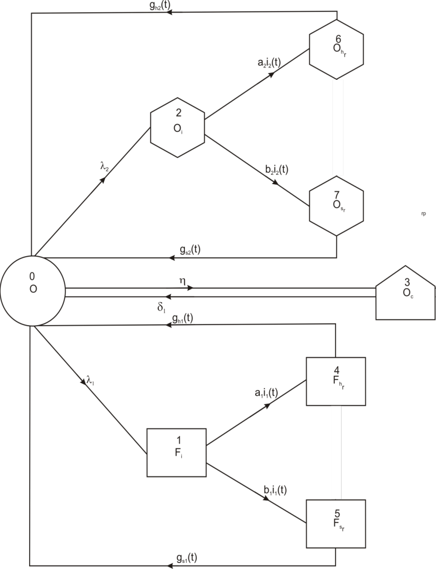 Figure 1
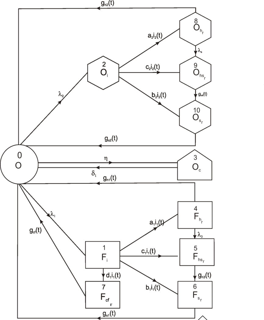 Figure 2
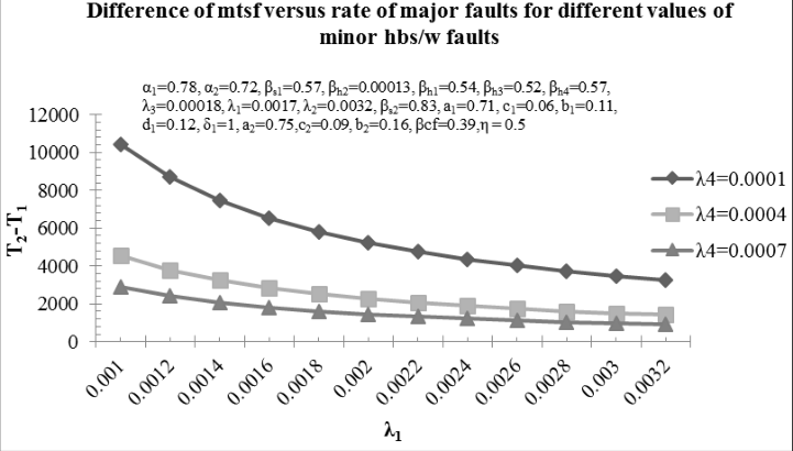 Figure 3
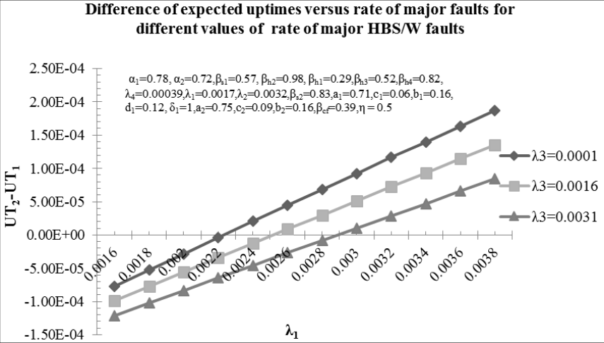 Figure 4
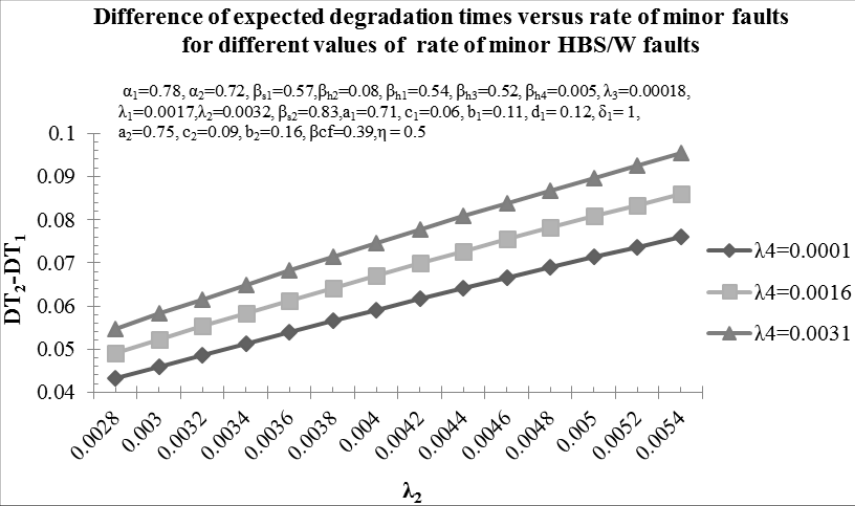 Figure 5
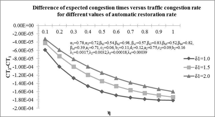 Figure 6
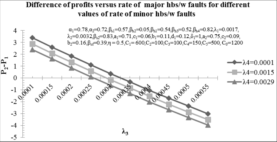 Figure 7
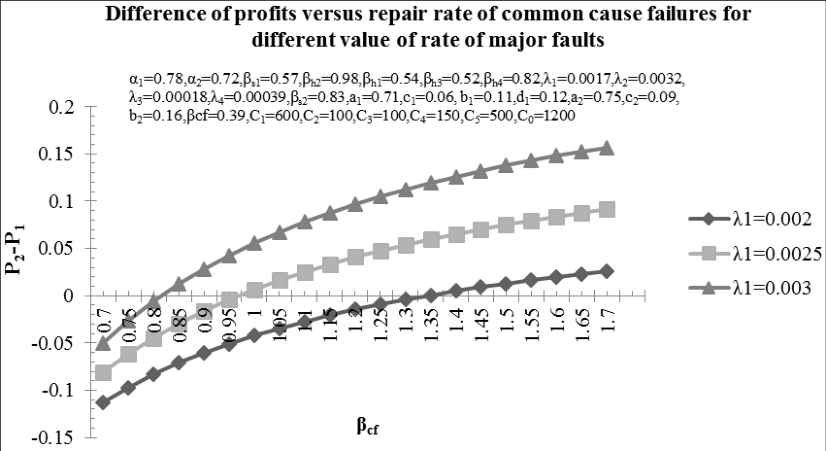 Fig. 8
Introduction
In the field of reliability, several researchers Arora [1] , garg and Kumar [2] , Goel et al. [3] and Gupta and Kumar [4] analyzed a large number of systems considering various aspects such as different failure modes, repairs, replacements, inspections and different operational stages. Murari and Goyal [10] studied reliability system with two types of repair facility. Gopalan et al. [3] did cost analysis of a system subject to on-line preventive maintenance and repair. Kumar and Mor [8] have given a probabilistic analysis of a sophisticated system with some warranted components considering two types of service facility and delay in warranty claims. Beside these a few researchers like Teng et al. [11] , Tumer and Smidts [12] , Welke et al. [13] , Kumar and Kumar [9] , Kumar and Kapoor [7] etc. discussed various types of hardware/software failures with different recovery policies while analyzing systems having both hardware and software components. Kumar and Kapoor [8] did the comparative analysis of stochastic models for a base transceiver system considering software based hardware failure and congestion of calls. Recently, Kumar and Kapoor [5] analysed a model on a base transceiver system onsidering hardware faults, software faults and congestion of calls. Thereafter, for the system Kumar and Kapoor [6] discussed a model considering hardware based software faults and catastrophic failures. It is pertinent to mentioned that the model developed for a system cannot be good for all its operational conditions/situations. However stakeholders are interested to judge which and when one model is better for the system with respect to different measures of system performance. Keeping this fact in view, in the present paper a comparative analysis has been done between the models for a base transceiver system given in [5] and [6] to investigate which and when a model is better for the system, respectively, in terms of their reliability, expected uptime/degradation times/congestion time and profit. A base transceiver system may fail or may not work satisfactorily on occurrence of some major or minor faults, common cause failures or network traffic congestion. When major/minor fault occurs the repair team first inspects whether there is hardware or software or hardware based software fault then recovery of the relevant component is done. In the first model given in [5] , only hardware faults, software faults and network traffic congestion are taken whereas in the model given in [6] , hardware based software failures and common cause failures are taken apart from considering occurrence of some minor or major faults in hardware/ software components and traffic congestion. In these models it is assumed that the minor fault leads to partial failure or degradation state whereas a major fault and common cause failure leads to complete failure of the system. On the basis of computed measures of system performance, comparison of the models with respect to their mean times to system failures, expected uptimes/degradation times and profits is made using graphs for some particular case and conclusions are drawn.
States of
States of
State Transition Diagram
For the model-I, a diagram presenting various states of transition of the system is shown in fig. 1 whereas for the model-II, various states are given in fig. 2. In both the diagrams the epochs of entry in to various states are regenerative points and hence all the states are regenerative states.
Transition probabilities and mean sojourn times
Various transition probabilities and mean sojourn times respectively for the Model-I and Model-II as given in [5] and [6] are as under. The mean sojourn time (µi) in the regenerative state i is defined as the time of stay in that state before transition to any other state. If T denotes the sojourn time in regenerative state i, then
Model-I
The unconditional mean time taken by the system to transit for any regenerative state j, when it is counted from epoch of entrance into that state i, is mathematically stated as mij = t qij(t) dt Thus, m01 By these transition probabilities, it can be verified that p01 + p02 + p03 = p14 + p15 + p16 + p17 = p28 + p29 + p2,10 = p40 + p45 = p80 +p89 = 1 p30 = p56 = p60 = p70 = p9, 10 = p10,0 = 1 The mean sojourn time (µi) in the regenerative state i is defined as the time of stay in that state before transition to any other state. If T denotes the sojourn time in regenerative state i, then
Measures of System Performance
For the purpose of comparison between the models following values of measures of performance of the system are taken from [5] and [6] : =N52/ D12 (Repair time only) where N1= µ0 + p02 µ2+ p03 µ3+ p02 (p26 µ6 + µ8p28 + p27µ7) N2= µ0 + p02 µ2+ p03 µ3+ p02 p28 µ8 + (p02 p28 p89 + p02 p29) µ9 + (p02 p28 p89 + p02 p29 + p02 p210) µ10 N11= µ0 N21= p02µ2+p02 p26µ6+p02 p27µ7 N31 = p03µ3 N41= p01µ1+p02µ2, N51= p01 p14µ4 + p01p15µ5 + p02p26µ6 + p02p27µ7, N22 = p02µ2 + p02 p28µ8 + p02 (p28 p89 + p29) µ9 + p02( p28 p89 + p29 + p210) µ10, N52= p01p14µ4 + (p01p14 p45+ p01p15) µ5+ (p01p14p45 + p01p15 +p01p16) µ6 + p01p17µ7 + p02p28µ8 + (p02p28p89 + p02p29)µ9 + (p02p28p89 + p02p29 + p02p210) µ10 D1 = p01 D11= µ0+ p01µ1+ p02µ2 + p03 µ3+ p01p14µ4 + p01p15µ5+ p02 p26µ6 + p02 p27 µ7 D12= µ0 + p01µ1 + p02µ2 + p03µ3 + p01p14µ4 + p01 (p14p45 + p15) µ5 + p01 (p14p45 + p15 + p16) µ6 + p01 p17µ7+ p02p28 µ8 + p02 (p28p89 + p29) µ9 + p02 (p28p89 + p29 + p210) µ10
Profit analysis
The expected profits of the system corresponding to model-I and model-II are:
Where C0 = revenue per unit uptime of the system C1= revenue per unit degradation time of the system C2 = revenue per unit congestion time of the system C3 = cost per unit time of inspection C4 = cost per unit time of repair C = cost of installation of the system
Graphical analysis
For graphical analysis the following particular case is considered: Fig. 3 shows the behavior of difference of mean times to system failure of the system i.e. T2-T1 with respect to the rate of occurrence of major faults (λ1) for different values rate of occurrence of minor hardware based software faults (λ4). The graph reveals that the difference of mean times to system failure of two models decreases with increase in the values of rate of occurrence of major faults and has lower values for higher values of the rate of minor hardware based software faults. This also concludes that that model II has more reliability than model I.
Fig 3
The curves in the fig. 4 shows the behavior of difference of the expected uptimes (UT2-UT1) with respect to the rate of occurrence of major fault of the system (λ1) for the different values of rate of occurrence of major hardware based software faults (λ3). It is evident from the graph that difference of expected uptimes increases with the increase in the values of rate of occurrence of major fault and has lower values for higher values of rate of occurrence of major hardware based software fault (λ3). From the fig. 4 it may also be observed that for λ3= 0.0001, difference of the expected uptime is < or = or > 0 according as λ1 is < or = or > 0.00223. Hence the Model I is better or equally good or worse than Model II whenever λ1 is < or = > 0.00223.Similarly, for λ3= 0.0016 and λ3=0.0031, difference of the expected uptimes is < or = or > 0 according as s λ1 is < or = or > 0.00252 and 0.00289 respectively. Thus, in these cases, Model I is better or equally good or worse than Model II whenever λ1 < or = or > 0.00252 and λ1 < or = or > 0.00289.
Fig 4
Fig. 5 shows the behavior of difference of the expected degradation times of the system i.e. DT2-DT1 on the basis of two models with respect to the rate of occurrence of minor faults (λ2) for different values of rate of occurrence of minor hardware based software faults (λ4). The graph reveals that the difference of expected degradation times of the two models increases with increase in the values of rate of occurrence of minor faults and has higher values for higher values of rate of occurrence of minor hardware based software faults. This shows that model II has more expected degradation time than model I. The curves in the fig. 7 shows the behavior of the difference of profits (P2-P1) with respect to the rate of occurrence of major hardware based software faults of the system (λ3) for the different values of rate of occurrence of minor hardware based software faults (λ4). It is evident from the graph that difference of profits decreases with the increase in the values of rate of occurrence of major hardware based software faults and has lower values for higher values of minor hardware based software faults. From the fig. 7 it may also be observed that for λ4 = 0.0001, the difference of profits is > or = or < 0 according as λ3 is < or = or > 0.000326. Hence the Model II is better or equally good or worse than Model I whenever λ3 < or = or >0.000326. Similarly, for λ4=0.0015 and λ4=0.0029, the profit difference is > or = or < 0 according as is λ3 < or = or > 0.00029 and 0.000258 respectively. Thus, in these cases, Model II is better or equally good or worse than Model I whenever λ3 < or = or > 0.00029 and λ3 < or = or >0.000258. The curves in the fig. 8 shows the behavior of the difference of profits (P2-P1) with respect to the repair rate of common cause failures ( f c ) for the different values of rate of occurrence of major faults (λ1). It is evident from the graph that difference of profits increases with the increase in the values of repair rate of common cause failures and has higher value for higher values of rate of occurrence of major faults. From the fig. 8 it may also be observed that for λ1=0.002 the difference of profits is < or = or > 0 according as f c is < = or > 1.34. Hence the Model I is better or equally good or worse than Model II whenever f c is < = or > 1.34. Similarly, for λ1=0.0025 and λ1=0.003 the difference of profits is < or = or > 0 according as is f c < or = or > 0.969 and 0.817 respectively. Thus, in these cases, Model I is better or equally good or worse than Model II whenever
Conclusion
From the comparative analysis it can be concluded that the difference of mean times to system failure of the models decreases with increase in the rate of occurrence of major faults and has lower values for higher values of rate of occurrence of minor hardware based software faults. It is also concluded that the model given in [6] has higher reliability than model given in [5] for some considered values of the parameters. It also revealed from the analysis that difference of expected uptimes increases with increase in the values of major faults and has lower values for higher values of rate of major hardware based software faults. It is also concluded that the difference of the expected degradation times increases with increase in the values of rate of occurrence of minor faults and has higher values for higher values of rate of minor hardware based software faults. It may also be concluded that expected degradation time of model given in [6] is more than model given in [5] for the given values of parameters. Further it is observed that difference of expected congestion times decreases with increase in the values of rate of network traffic congestion and has higher values for higher values of automatic network restoration rate. It also reveals that expected congestion time of model given in [6] is less than model given in [5] . Also cut-off points for various parameters of importance can be obtained for differences expected uptimes and profits of the models given in [5] and [6] to suggest the stakeholders which model is better and under what conditions.
Figures and tables from the paper
References
13 in the original paper- Arora JR. Reliability of several standby priority redundant systems, IEEE Transactions on Reliability, 1977; 26(4):290-293.
- Garg RC, Kumar A. A complex system with two types of failure and repair, IEEE Transactions on Reliability, 1977; 26(4):299-300.
- Goel LR, Sharma GC, Gupta R. Reliability analysis of a system with preventive maintenance and repair, Microelectronics Reliability, 1986; 26:429-433.
- Gupta ML, Kumar A. On profit consideration of a maintenance system with minor repair, Microelectronics Reliability, 1983; 23:437-439.
- Kumar R, Kapoor S. Cost-benefit analysis of a reliability model for a base transceiver system considering hardware/software faults and congestion of calls. International Journal of Science and Technology. 2012; 4(6):13-23.
- Kumar R, Kapoor S. Economic and performance evaluation of stochastic model on a base transceiver system considering various operational modes and catastrophic failures. Journal of Mathematics and Statistics. 2013; 9(3):198-207.
- Kumar R, Kapoor S. Profit evaluation of a stochastic model on Base Transceiver system considering software based hardware failures and congestion of calls. International Journal of Application or Innovation in Engineering and Management. 2013; 2(3):554-562.
- Kumar R, Kapoor S. Comparative performance analysis of two reliability models for one unit base transceiver system having software based hardware failures and congestion of calls, Proceedings of the International Conference on Information & Mathematical Sciences held at Baba Farid College of Engineering & Technology, Bathinda, Punjab, 2013, 397-401.
- Kumar R, Kumar M. Performance and cost-benefit analysis of a hardware-software system considering hardware based software interaction failures and different types of recovery. International Journal of Computer Application. 2012; 78(2):29-35.
- Kumar R, Mor S. Probabilistic analysis of a sophisticated system with some warranted components considering two types of service facility and delay in warranty claims. Caledonian Journal of Engineering. 2011; 7(2):21-27.
- Teng X, Pham H, Jeske DR. Reliability modeling of hardware and software interactions, and its applications, IEEE Transactions on Reliability, 2006; 55(4):571-57.
- Tumer IY, Smidts CS. Integrated design-stage failure analysis of software driven hardware systems, IEEE Trans on Computers, 2011; 60(8):1072-1084.
- Welke SR, Johnson BW, Aylor JH. Reliability modeling of hardware/software systems, IEEE Transactions on Reliability, 1995; 44(3):413-418.