
Research article · 2020 · Full text
International Journal of Statistics and Applied MathematicsArima model in forecasting share prices
Volume 5(4) · Pages 147–151
Research areasStock Market Forecasting MethodsForecasting Techniques and Applications
Abstract
Author-writtenThe fluctuation in share price of a particular company is of great concern for investors who want to invest in that particular company. These fluctuations are analysed in detail using various statistical techniques. Analysts make use of historical data to predict the trends, patterns in the data, or forecast the process behaviour either within the range or outside the range of the observed data so that investors can have an idea about the market behaviour. Amongst the various techniques used for forecasting, a time series forecasting tool called ARIMA (Auto Regressive Integrated Moving Average) method has been used from time to time. For this, R programming software is used which is useful for visualization, statistical computing, scientific inference, and graphical interface. R Studio is a free and powerful integrated development environment for R language which allows the user to implement ARIMA Model.The data of the share prices for the past two years of Star Cement Ltd. has been collected and trained using ARIMA model with different parameters. The test criterion like Akaike Information Criterion is applied to analyse the accuracy of the model. The one with the least AIC is chosen. The model is then used to forecast the performance of the stock for the next ten data points.
Summary
Source-checkedPlain-language reading of the full paper, prepared with AI and checked against the text. Each point links to the authors' own words.
Why it matters
- Share price fluctuations are a significant concern for investors looking to invest in specific companies. View evidence ↗
- Analysts use historical data to forecast market behavior and trends to help investors make informed decisions. View evidence ↗
- Time Series Analysis is a scientific technique that processes verifiable historical data to evaluate future trends. View evidence ↗
The question
- The study aims to use the ARIMA forecasting tool to predict the share prices of Star Cements Ltd. View evidence ↗
What they did
- The researchers collected closing share price data for Star Cement from April 29, 2018, to April 24, 2020. View evidence ↗
- R programming software was used for statistical computing, visualization, and implementing the ARIMA model. View evidence ↗
- The Akaike Information Criterion (AIC) was used to determine model accuracy, with the model exhibiting the lowest AIC being selected. View evidence ↗
- The data frequency was set to 5 days to reflect the standard operating days of the market. View evidence ↗
What they found
- The Augmented Dickey-Fuller test resulted in a p-value of 0.5091, indicating that the original share price data was not stationary. View evidence ↗
- A Durbin-Watson test on first-order differenced data yielded a p-value of 0.849, confirming the absence of autocorrelation. View evidence ↗
- Among the manually tested models, ARIMA (0, 1, 0) was identified as the best fit due to having the lowest AIC of 2159.3. View evidence ↗
- The Ljung-Box test for the ARIMA (0, 1, 0) model residuals showed a p-value of 0.3243, supporting the model's adequacy. View evidence ↗
- The model forecasted the next ten data points to increase linearly from 100.00 to 101.80. View evidence ↗
What it means
- The authors conclude that forecasting the stock price of Star Cement provides useful insights for making wise future investments. View evidence ↗
- A limitation of the study is that it does not account for various external factors affecting stock prices, which may violate the linearity assumption of the model. View evidence ↗
Visual summary
2 visualsIllustrations explain the paper; charts are replotted from the paper's own table values.
ARIMA Model Selection Process
AI-generated conceptual illustration (a digital stock market price line graph on a computer screen). It explains the idea and does not show study data.
View source evidence ↗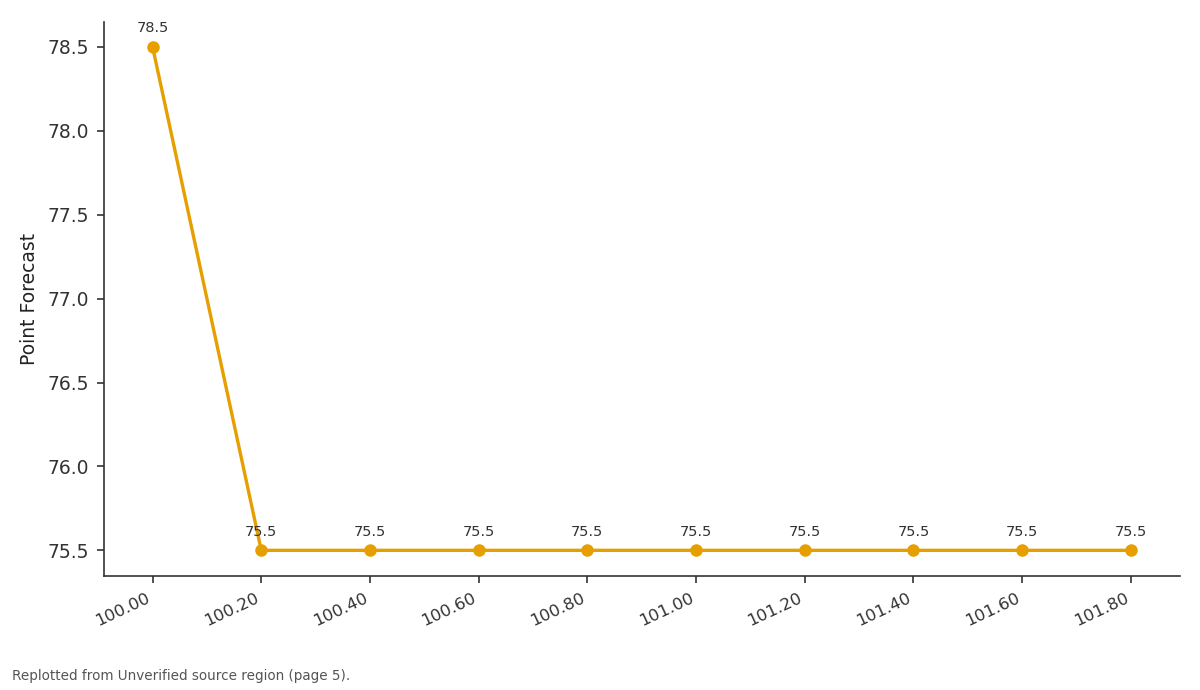
Point Forecast: 100.00 vs 100.20 vs 100.40 vs 100.60 vs 100.80
Replotted from a table (page 5) of the original paper. Every bar is the paper's own table value.
View source evidence ↗Figures & tables
From the original paper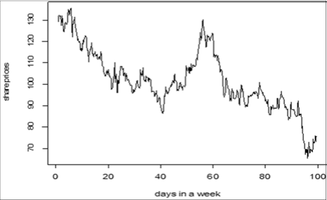 Figure 1
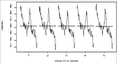 Figure 2
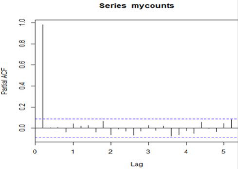 Figure 3
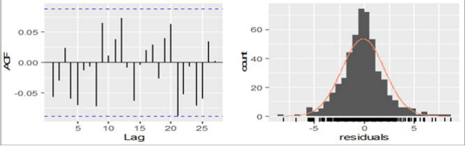 Figure 4
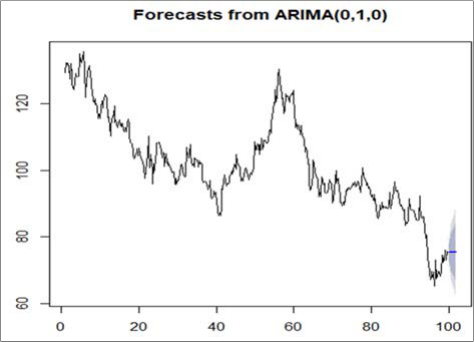 Figure 5
Introduction
Most of the people interested in investment consider stock market as a means of gambling. They hardly consider it as a means of investment. Even when the markets have crashed from their all time highs, people are still not ready to encash this opportunity. They remain in a dilemma that the market will go down to zero, which quite ironically would never happen. Shares and stocks in their literal sense represent ownership of the business. Share/stock market is a part of the capital market which comprises of the Money market and the Capital market. In Money Market short term financial instruments (Treasury Bills, Bank Deposits, Commercial Papers and Treasury Certificates) are issued and traded whereas Capital Market deals only in Long Term financial instruments like bonds and securities. Generally participants in money market raise money to meet working capital needs or such short term financial needs whereas money raised via capital market is used for long term financial needs. Governments or companies issue bonds or stocks in the market to raise money which are used for fixed investment projects like infrastructure projects or building plants, buying machines etc. So both money market and capital market work in harmony in the nation building process. In fact their existence is not mutually exclusive rather they work hand in hand. Moreover, it is the stock exchange that provides liquidity in the capital market, as such it's very important for development of the capital market as a whole. Stock Exchange is the platform where trading of securities takes place via computers, telephone, fax, trading floor etc. Initially the companies raise money by issuing their securities in the primary market after the subscription of which they get listed in the stocks market. Generally there are three main forms of investment -Real Estate, Commodities and Securities. People park most of their money in the first two instruments in the form of land, flats, gold, silver etc, but are afraid to invest in securities especially in stocks. They remain fearful by seeing the constant fluctuations in the stock prices but remain ignorant of the fact that if their real estate properties would have been listed in a similar exchange the scenario would have been the same. People consider stocks as risky but the fact is one can minimize this risk by knowing about the business in which they are investing. So the larger question remains as to how an investor educates himself about the stock market? How will he predict the market? Well, timing the market is next to impossible but one can definitely predict the market through various scientific techniques available. One of such techniques is Time Series Analysis. This method collects verifiable data, processes it and then evaluates future on the basis of the results. Time series data are collected over a period of time and in a particular sequence. It is considered as an important tool for forecasting the trend and provides adequate guidance to the investors in the forms of charts and graphs.
Literature Review
Devi et al. (2013) [2] in their paper used data mining tools and analytical technologies to do a quantifiable amount of research to explore new approach for the investment decisions. The stock data for the past five years has been collected and trained using ARIMA model with different parameters. The test criterions like Akaike Information Criterion Bayesian Information Criterion (AICBIC) are applied to predict the accuracy of the model. The performance of the trained model is analyzed and it also tested to find the trend and the market behavior for future forecast. Kamalakannan et al. (2018) [6] in their paper used the Time Series Forecasting methodology for predicting and visualizing the predictions which were based on the technical analysis using historic data and ARIMA Model. Autoregressive Integrated Moving Average (ARIMA) model has been used extensively in the field of finance and economics as it is known to be robust, efficient and has a strong potential for short-term share market prediction. Angadi and Kulkarni (2015) [1] in their work proposeda prediction model for the time series stock market data. This model was supposed to automate the process of change of stock price indices based on technical analysis and provided assistance for financial specialists to choose better timing for purchasing and selling stocks. Data mining techniques were used to develop the prediction model and R programming language was used for visualization of results. Varghese et al., (2016) [8] argued that Since stock market data are highly time-variant and are normally in a nonlinear pattern, predicting the future price of a stock is highly challenging. Prediction provides knowledgeable information regarding the current status of the stock price movement. Thus this can be utilized in decision making for customers in finalizing whether to buy or sell the particular shares of a given stock. Many researchers have been carried out for predicting stock market price using various data mining techniques. The past data of the selected stock will be used for building and training the models. The results from the model will be used for comparison with the real data to ascertain the accuracy of the model. Viswam and Reddy (2018) [9] predicted the stock trends in an effective manner which can minimize the risk of investing and maximize profit. In their paper, they used the Time Series Forecasting methodology for predicting and visualizing the predictions. Our focus for prediction will be based on the technical analysis using historic data and ARIMA Model. Autoregressive Integrated Moving Average (ARIMA) model has been used extensively in the field of finance and economics as it is known to be robust, efficient and has a strong potential for short-term share market prediction. Subashinil and Karthikeyan (2018) [7] in their paper proposed a model for forecasting the stock market trends based on the technical analysis using historical stock market data and ARIMA model. This model processed future stock price indices and provides assistance for financial specialists to purchasing and/or selling of stocks at the right time. The forecast results are visualized using R programming language.
Results of ARIMA model have a strong potential for shortterm prediction of stock market trends. Dhanalaxmi et al. (2016) [3] used the statistical methods such as AR model and Kalman filter for solving highly non-linear problems. In their paper, an attempt is made to develop practical methods of non-linear time series by introducing soft computing technique as Chaos theory and Neural Network. Using the stock market data input to various models, the applicability and accuracy of the proposed methods are discussed with comparison of results. Iwok and Okoro (2016) [4] seek to forecast stocks of the Nigerian banking sector using probability multivariate time series models. The study involved the stocks from six different banks that were found to be analytically interrelated. Stationarity of the six series were obtained by differencing. Model selection criteria were employed and the best fitted model was selected to be a vector autoregressive model of order 1. The model was subjected to diagnostic checks and was found to be adequate. Consequently, forecasts of stocks were generated for the next two years. Jadhav et al. (2015) [5] used neural networks (ANNs) as a flexible computing frameworks and universal approximates that can be applied to a wide range of time series forecasting problems with a high degree of accuracy for the convenience of predicting the futuristic value in share market and give a better future scope for investment. Thus from an exhaustive study of the literature the following objective is formulated.
Objective:
The basic objective in this study is to use a forecasting tool like ARIMA for predicting the share prices of a particular company. The data for the same is collected from Star Cements Ltd.
Method and Methodology
One of the models of Time Series Analysis Technique which is used in this paper is ARIMA Model. Autoregressive Integrated Moving Average (ARIMA) model gives us more accurate results. This is one of the most popular models to predict linear time series data. This model was introduced by Box and Jenkins (hence also known as Box-Jenkins model) in 1960s for forecasting a variable ARIMA stands for Auto Regression Integrated Moving Average and is specified by three ordered parameters (p, d, q). Here p is the order of the autoregressive model (number of time lags), d is the degree of differencing(number of times the data have had past values subtracted), q is the order of moving average model. Before an ARIMA model is built, it is essential to check whether the data is stationary i.e. The mean of the time series should not be a function of time which means it should be constant, the variance of the time series should not be a function of time, the covariance of the ith term and the (i+m) th term should not be a function of time. The stationarity of the data series can be checked either by checking the correlogram or the autocorrelation function (ACF) and partial ACF (PACF) of the time series data. In ARIMA model the future value of the variable is expressed as a linear combination of past values and past errors. ARIMA model is a generalization of Auto Regressive (AR) and Moving Average (MA) including the notion stationary (integration).Moving Average model (MA) A moving average (MA) process is a modest class of time series model. It consists of past error ( ) multiplied by a constant (coefficients) where a simple 1 st order MA process can be expressed as,
wherec1,,c2,c3,....cqare the parameters of the model, c0 is aconstant,vt-1, vt-2, vt-3...vt-q are lagged values of errorand vt white noise i.e. 2 t v N(0, ) . ( 1) is moving average model of order 'q'. It is basically a linear combination of past error processes such that depends on the current and previous values of past error terms. Auto Regressive Method (AR) This is also known as autoregressive process AR(P) that is a process in which existing value of a variable is a linear combination of past values and an error term.
1 st order Autoregressive model, denoted by AR ( 1) is expressed as,
(2) is autoregressive model of order 'P'.d0 and djare (AR) coefficients and Y t-jare the lagged values of the series Yt, t~ i. i. d (0, 2). Combining both MA (Q) and AR (P) an autoregressive moving average ARMA (P, Q) process is defined.
Where 'I' is order of differencing transforming the series into a stationary, p is the order of autoregressive process and q represent moving average process order. Stationary process is one of the key concepts of a time series, so taking difference to make stationary an ARMA (P, Q) process is called auto regressive integrated moving average and denoted by ARIMA (P, I, Q). The data does not show exponential description nor is there trend present and is very typical of seasonal fluctuations. There is a an upward and then a downward trend and the values did not vary over time around a constant mean and variance which is the basic requirement for the stationarity of a series. This graph is zoomed out using the following function to have a better perspective of the fluctuations. The variations within each day is visible using the following function. Month plot (my counts, labels=1:5, xlab="days in a week") The month plot calculates the average for each time unit. The line in the middle is the mean of that particular day. As is visible in the data the average price appears constant throughout the various days of a particular week. Now the stationarity of the data is checked. Itis achieved by differencing which is obtained by subtracting the previous value from the current value. Depending on the complexity of the series, sometimes more than one differencing may be needed. This is actually the value the value of d, which is the minimum number of differencing needed to make the series stationary. And if the time series is already stationary, then d = 0. The right order of differencing is the minimum differencing required to get a near-stationary series which roams around a defined mean and the ACF plot reaches to zero fairly quick. This is done by using Augmented Dicky Fuller test given by the following function: adf. test (mycounts) Augmented Dickey-Fuller Test data: my counts Dickey-Fuller = -2.1633, Lag order = 7, pvalue = 0.5091Alternative hypothesis: stationary As the p value is greater than 0.05 this suggests that we accept the null hypothesis of no stationarity in the data. This is also confirmed using the ACF and PACF plots. ACF (PACF) of the share price data.>acf (mycounts)>pacf (my counts) The plots too suggest that the data is not stationary as the values cross the threshold values at every point. Therefore to ensure that the data is stationary we take the difference of 1 st order using Durbin-Watson test. This is ensured using the following function: Dwtest (my counts [-495] ~my counts [-1]) data: my counts[-495] ~ my counts[-1] DW = 2.0967, p-value = 0.849 alternative hypothesis: true autocorrelation is greater than 0As p >.05 it confirms no autocorrelation is there. With the ACF showing no autocorrelation, we move ahead to fit an ARIMA model using trial and error method. The choice of the best model depends on the AIC criterion. Among the various models tested the one with the lowest AIC is fitted. The required number of AR terms can be detected by inspecting the Partial Autocorrelation (PACF) plot. Partial autocorrelation can be imagined as the correlation between the series and its lag, after excluding the contributions from the intermediate lags. So, PACF sort of conveys the pure correlation between a lag and the series. Just like how we looked at the PACF plot for the number of AR terms, we can look at the ACF plot for the number of MA terms. An MA term is technically, the error of the lagged forecast. The ACF tells how many MA terms are required to remove any autocorrelation in the stationarized series. The ARIMA model is obtained as follows using the hit and trial method. Thus from the various models tried manually it is seen that ARIMA (0, 1, 0) is the best with the least AIC which is 2159.3. This is also confirmed using the following function of ARIMA
ARIMA model in words
ARIMA model in words
Auto. arima (mycounts, trace=T, stepwise=F, approximation=F)
This generates a list of multiple models out of which one of the following result is obtained. Series: my counts ARIMA (0,1,0)(1,0,0) [5] Coefficients: sar1 -0.
Figures and tables from the paper
References
8 in the original paper- Angadi MC, Kulkarni AP. Time Series Data Analysis for Stock Market Prediction using Data Mining Techniques with R. International Journal of Advanced Research in Computer Science, 2015, 6(6).
- Devi BU, Sundar D, Alli P. An effective time series analysis for stock trend prediction using ARIMA model for nifty midcap-50.International Journal of Data Mining & Knowledge Management Process. 2013; 3(1):65.
- DhanalaxmiM, Chakradhar B, Sreedhar B. Time Series Prediction of Stock market data by using Chaos theory and Neural Network, International Journal of Scientific & Engineering Research. 2016; 7:3.
- Iwok AI, Okoro CB. Forecasting Stocks with Multivariate Time Series Models, International Journal of Mathematics and Statistics Invention (IJMSI). 2016; 4(9):32-44.
- Jadhav S, Kakade S, Utpat K, Deshpande H. IndianShare Market Forecasting with ARIMA Model. International Journal of Advanced Research in Computer and Communication Engineering. 2015; 4(11):334-336.
- Kamalakannan SenguptaI, Chaudhury S. StockMarket Prediction using Time Series Analysis, Computing Communications and Data Engineering Series. 2018; 1:3.
- Varghese A, Tarhen H, Shaikh A, Banik P, Ramadasi A. Stock Market Prediction Using Time Series. International Journal on Recent and Innovation Trends in Computing and Communication. 2016; 4(5):427-430.
- Viswam N, Reddy GS. Stock market prediction using time series analysis. International Journal of Statistics and Applied Mathematics. 2018; 3(1):465-469.