
Research article · 2020 · Full text
International Journal of Statistics and Applied MathematicsSelection of Bayesian skip lot sampling plan-3 with conditional repetitive group sampling plan using Trignometric Ratio Method
Volume 5(4) · Pages 196–200
Research areasAdvanced Statistical Process MonitoringManufacturing Process and Optimization
Abstract
Author-writtenAcceptance sampling plans on the basis of Bayesian methodology can be taken when the innovator has prior knowledge on the process fluctuation to take a opinion about the disposition of the lot. Bayesian sampling plan has a clear picture on the influences associated with the selection of appropriate prior distribution. This paper describes new method for Bayesian Skip Lot Sampling Plan-3 with Conditional Repetitive Group Sampling Plan using Trigonometric Ratio Methods. Tables and numerical examples are also provided.
Summary
Source-checkedPlain-language reading of the full paper, prepared with AI and checked against the text. Each point links to the authors' own words.
Why it matters
- Acceptance sampling serves as a defensive mechanism to prevent the depreciation of product quality. View evidence ↗
- Bayesian sampling plans are considered more powerful than current plans because they can reduce surveillance costs and improve sample size effectiveness. View evidence ↗
- Skip-lot sampling allows quality assessment by reviewing only a limited proportion of very large conforming lots. View evidence ↗
The question
- The study aims to construct a new method for a Bayesian Skip Lot-3 sampling plan using a Conditional Repetitive Group Sampling reference plan indexed via the trigonometric ratio method. View evidence ↗
What they did
- The trigonometric ratio method works by comparing sections of the Operating Characteristic (OC) curve against a corresponding ideal OC curve. View evidence ↗
- The method involves creating a line between the Acceptable Quality Level (AQL) and a 50% probability of acceptance; a smaller angle (Ɵ) indicates the curve is closer to the ideal OC curve. View evidence ↗
What they found
- The study provided parametric values for various configurations; for example, with f=1/4, s=2, i=2, and icrgs=1, the value for a 0.05 probability level is 0.8751. View evidence ↗
- Operating ratio values were tabulated for different alpha and beta combinations; for f=1/2, s=2, i=2, icrgs=1, and alpha=0.05, the operating ratio is 16.6915. View evidence ↗
What it means
- The authors state that this enhanced technique is applicable not only in production but also in the employment sector. View evidence ↗
Visual summary
2 visualsIllustrations explain the paper; charts are replotted from the paper's own table values.
OC Curve Comparison
AI-generated conceptual illustration (A mathematical coordinate system with geometric curves). It explains the idea and does not show study data.
View source evidence ↗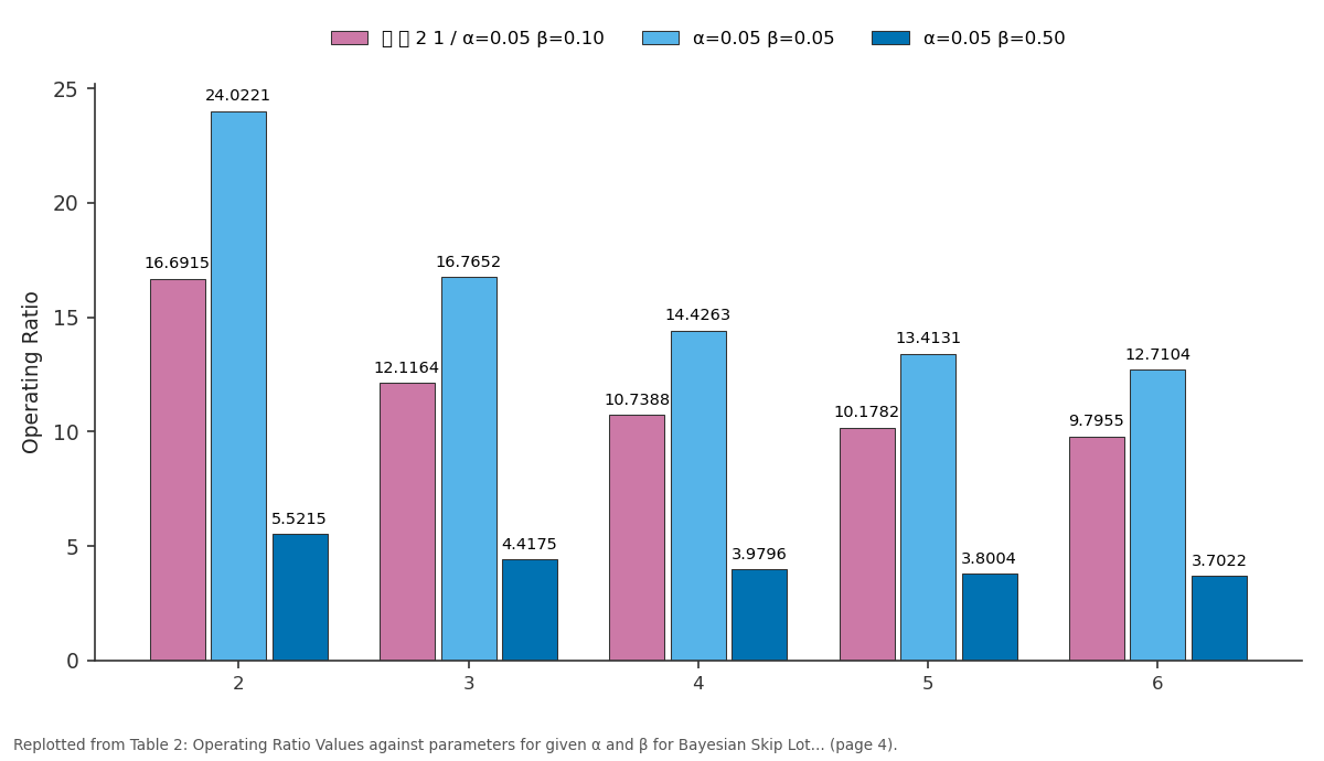
2 1 / α=0.05 β=0.10 and α=0.05 β=0.05 and more: 2 vs 3 vs 4 vs 5 vs 6
Replotted from Table 2 (page 4) of the original paper. Every bar is the paper's own table value.
View source evidence ↗Figures & tables
From the original paper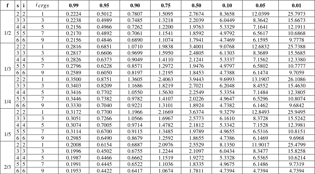 Table 1
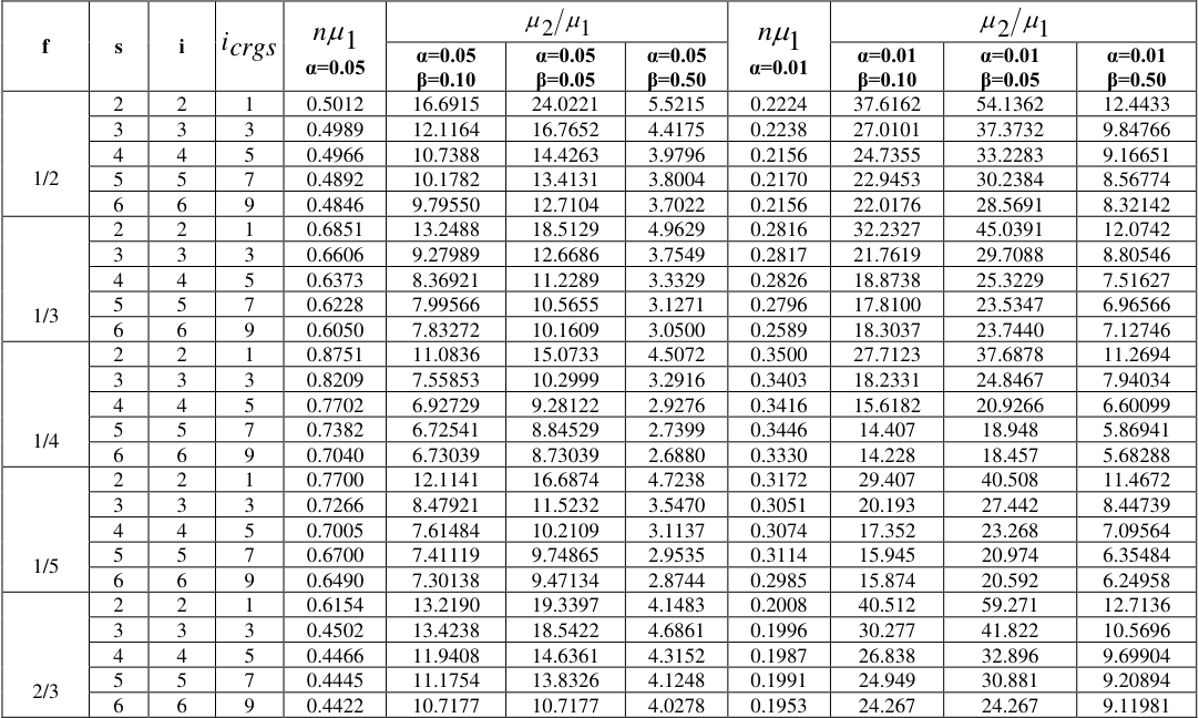 Table 2
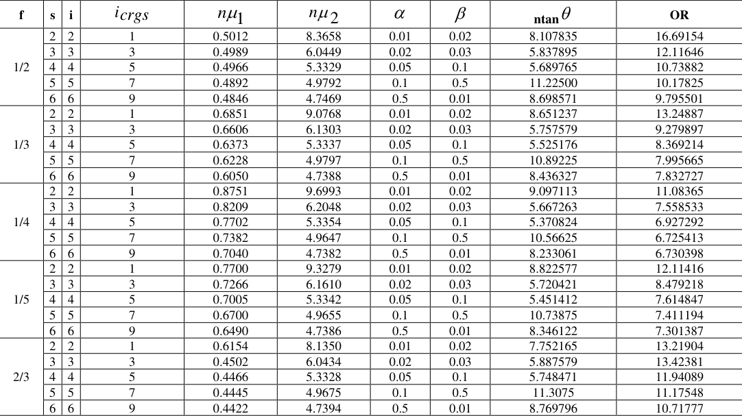 Table 3
Introduction
Acceptance Sampling is undoubtedly a opposing part, intiated as defensive accessory against the intimidation of depreciation in quality. Review of lot and ultimate product is fundamental to establish acceptable quality. Literally the concept of sampling inspection pays extra consideration to revamp the quality and lessen cost in terms of minimal sample size. Under this system manufactures are capable to take inventive production with the use of Bayesian Sampling Plan that is more powerful than current sampling plan, taking lesser surveillance cost and effectiveness over sample size.
Bayesian Acceptance Sampling distribution access is combined with the usage of the prior process history for the choice of diffusion (Gamma- Poisson, Beta-Binomial) to explain the random variations involved in acceptance sampling. Bayesian Sampling Plans requires the customer to indicate exceptionally the distribution of the defectives from lot to lot. The skip-lot Sampling methodology was advanced from the approach of continuous sampling plan, that is the quality authority of a product can be revised over the review of limited proportion of very large-conforming lots. The reference plan advanced for commerce purpose to overcome the inspected items of production towards producer risks and consumer risks, alpha and beta risks continued on lot-by-lot inspection.
Dodge and Perry (1971) [2] establish the operation of Skip lot Sampling to the condition in one by one lot to be inspected is sampled confer to a few lot inspection plan is nominated as Skip lot Sampling Plan-2. Parker and Kessler (1981) [7] have altered the extant form of Skip lot Sampling Plan-2 under the principles in which at least one lot is consistently sampled from a construction of lot. Vijayaraghavan (1990) [11] described the Skip Lot Sampling Plan-3 which is also an extension of Skip Lot Sampling Plan -2 uses certain elementary methods of continuous sampling. According to Hald (1981) [3] contributed an admirable relation and classical Bayesian theory and procedure for attributes of acceptance sampling.
Calvin (1984) [1] has examined clearly and concisely the meaning of ‘how and when to perform Bayesian Acceptance Sampling’. Shankar and Mohapatra (1984) [9] advanced a modern sampling plan, it is an development of classical Repetitive Group Sampling Plan and nominated as Conditional Repetitive Group Sampling (CRGS) Plan. Kuralmani (1992) [5] made some improvement on Repetitive Group and certain relevant Conditional Sampling Plans. Latha (2002) [6] has explained the probability of acceptance for the Bayesian Single Sampling plan.
Maths 2020; 5(4): 196-200 S Jayalakshmi Assistant Professor, Department of Statistics, Bharathiar University, Coimbatore, Tamil Nadu, India Neena Krishna PK Ph.D., Research Scholar, Department of Statistics, Bharathiar University, Coimbatore, Tamil Nadu, India S Jayalakshmi Assistant Professor, Department of Statistics, Bharathiar University, Coimbatore, Tamil Nadu, India http://www.mathsjournal.com (i.e. =0.05 and =0.50, =0.05 and =0.10, =0.05 and =0.05). The major steps are as follows: 2 1 1. Find the operating ratio 2 1 2. Using the determined value of , applied the value from table 2 which is equal or just greater than the observed operating ratio. 3.
| f | s | i | icrgs | n 1 α=0.05 | 2 1 | — | — | n 1 α=0.01 | 2 1 | — | — |
|---|---|---|---|---|---|---|---|---|---|---|---|
| α=0.05 β=0.10 | α=0.05 β=0.05 | α=0.05 β=0.50 | α=0.01 β=0.10 | α=0.01 β=0.05 | α=0.01 β=0.50 | ||||||
| 1/2 | 2 | 2 | 1 | 0.5012 | 16.6915 | 24.0221 | 5.5215 | 0.2224 | 37.6162 | 54.1362 | 12.4433 |
| 3 | 3 | 3 | 0.4989 | 12.1164 | 16.7652 | 4.4175 | 0.2238 | 27.0101 | 37.3732 | 9.84766 | |
| 4 | 4 | 5 | 0.4966 | 10.7388 | 14.4263 | 3.9796 | 0.2156 | 24.7355 | 33.2283 | 9.16651 | |
| 5 | 5 | 7 | 0.4892 | 10.1782 | 13.4131 | 3.8004 | 0.2170 | 22.9453 | 30.2384 | 8.56774 | |
| 6 | 6 | 9 | 0.4846 | 9.79550 | 12.7104 | 3.7022 | 0.2156 | 22.0176 | 28.5691 | 8.32142 | |
| 1/3 | 2 | 2 | 1 | 0.6851 | 13.2488 | 18.5129 | 4.9629 | 0.2816 | 32.2327 | 45.0391 | 12.0742 |
| 3 | 3 | 3 | 0.6606 | 9.27989 | 12.6686 | 3.7549 | 0.2817 | 21.7619 | 29.7088 | 8.80546 | |
| 4 | 4 | 5 | 0.6373 | 8.36921 | 11.2289 | 3.3329 | 0.2826 | 18.8738 | 25.3229 | 7.51627 | |
| 5 | 5 | 7 | 0.6228 | 7.99566 | 10.5655 | 3.1271 | 0.2796 | 17.8100 | 23.5347 | 6.96566 | |
| 6 | 6 | 9 | 0.6050 | 7.83272 | 10.1609 | 3.0500 | 0.2589 | 18.3037 | 23.7440 | 7.12746 | |
| 1/4 | 2 | 2 | 1 | 0.8751 | 11.0836 | 15.0733 | 4.5072 | 0.3500 | 27.7123 | 37.6878 | 11.2694 |
| 3 | 3 | 3 | 0.8209 | 7.55853 | 10.2999 | 3.2916 | 0.3403 | 18.2331 | 24.8467 | 7.94034 | |
| 4 | 4 | 5 | 0.7702 | 6.92729 | 9.28122 | 2.9276 | 0.3416 | 15.6182 | 20.9266 | 6.60099 | |
| 5 | 5 | 7 | 0.7382 | 6.72541 | 8.84529 | 2.7399 | 0.3446 | 14.407 | 18.948 | 5.86941 | |
| 6 | 6 | 9 | 0.7040 | 6.73039 | 8.73039 | 2.6880 | 0.3330 | 14.228 | 18.457 | 5.68288 | |
| 1/5 | 2 | 2 | 1 | 0.7700 | 12.1141 | 16.6874 | 4.7238 | 0.3172 | 29.407 | 40.508 | 11.4672 |
| 3 | 3 | 3 | 0.7266 | 8.47921 | 11.5232 | 3.5470 | 0.3051 | 20.193 | 27.442 | 8.44739 | |
| 4 | 4 | 5 | 0.7005 | 7.61484 | 10.2109 | 3.1137 | 0.3074 | 17.352 | 23.268 | 7.09564 | |
| 5 | 5 | 7 | 0.6700 | 7.41119 | 9.74865 | 2.9535 | 0.3114 | 15.945 | 20.974 | 6.35484 | |
| 6 | 6 | 9 | 0.6490 | 7.30138 | 9.47134 | 2.8744 | 0.2985 | 15.874 | 20.592 | 6.24958 | |
| 2/3 | 2 | 2 | 1 | 0.6154 | 13.2190 | 19.3397 | 4.1483 | 0.2008 | 40.512 | 59.271 | 12.7136 |
| 3 | 3 | 3 | 0.4502 | 13.4238 | 18.5422 | 4.6861 | 0.1996 | 30.277 | 41.822 | 10.5696 | |
| 4 | 4 | 5 | 0.4466 | 11.9408 | 14.6361 | 4.3152 | 0.1987 | 26.838 | 32.896 | 9.69904 | |
| 5 | 5 | 7 | 0.4445 | 11.1754 | 13.8326 | 4.1248 | 0.1991 | 24.949 | 30.881 | 9.20894 | |
| 6 | 6 | 9 | 0.4422 | 10.7177 | 10.7177 | 4.0278 | 0.1953 | 24.267 | 24.267 | 9.11981 |
Table text extracted from the original PDF; superscript letters are shown inline. The original table image is below.
View original table image
Also find the values of n 1 𝑎𝑛𝑑 n 2 from the table 1 Pradeepa Veerakumari (2009) [8] has explained the evaluation of the performance measures for Bayesian conditional repetitive group sampling plan indexed through the quality levels. Suresh and Umamaheshwari (2014) [10] has evaluated the optimal design of Bayesian Skip-Lot Sampling Plan-2 with Conditional Repetitive Group Sampling Plan indexed through minimum angle method. In the present study, a new method for Bayesian Skip Lot -3 with Conditional Repetitive Group Sampling as reference plan indexed through trigonometric ratio method is constructed. 2. Conditions for the Application of Sampling Plan 1.
| f | s | i | icrgs | 0.99 | 0.95 | 0.90 | 0.75 | 0.50 | 0.10 | 0.05 | 0.01 |
|---|---|---|---|---|---|---|---|---|---|---|---|
| 1/2 | 2 | 2 | 1 | 0.2224 | 0.5012 | 0.7807 | 1.5095 | 2.7674 | 8.3658 | 12.0399 | 25.7973 |
| 3 | 3 | 3 | 0.2238 | 0.4989 | 0.7485 | 1.3218 | 2.2039 | 6.0449 | 8.3642 | 15.6673 | |
| 4 | 4 | 5 | 0.2156 | 0.4966 | 0.7262 | 1.2200 | 1.9763 | 5.3329 | 7.1641 | 12.1911 | |
| 5 | 5 | 7 | 0.2170 | 0.4892 | 0.7061 | 1.1541 | 1.8592 | 4.9792 | 6.5617 | 10.6868 | |
| 6 | 6 | 9 | 0.2156 | 0.4846 | 0.6890 | 1.1074 | 1.7941 | 4.7469 | 6.1595 | 9.7778 | |
| 1/3 | 2 | 2 | 1 | 0.2816 | 0.6851 | 1.0710 | 1.9838 | 3.4001 | 9.0768 | 12.6832 | 25.7388 |
| 3 | 3 | 3 | 0.2817 | 0.6606 | 0.9699 | 1.5950 | 2.4805 | 6.1303 | 8.3689 | 15.5685 | |
| 4 | 4 | 5 | 0.2826 | 0.6373 | 0.9049 | 1.4110 | 2.1241 | 5.3337 | 7.1562 | 12.3380 | |
| 5 | 5 | 7 | 0.2796 | 0.6228 | 0.8571 | 1.2972 | 1.9476 | 4.9797 | 6.5802 | 10.7777 | |
| 6 | 6 | 9 | 0.2589 | 0.6050 | 0.8197 | 1.2195 | 1.8453 | 4.7388 | 6.1474 | 9.7059 | |
| 1/4 | 2 | 2 | 1 | 0.3500 | 0.8751 | 1.3605 | 2.4063 | 3.9443 | 9.6993 | 13.1907 | 26.1086 |
| 3 | 3 | 3 | 0.3403 | 0.8209 | 1.1686 | 1.8219 | 2.7021 | 6.2048 | 8.4552 | 15.4630 | |
| 4 | 4 | 5 | 0.3416 | 0.7702 | 1.0550 | 1.5630 | 2.2549 | 5.3354 | 7.1484 | 12.3805 | |
| 5 | 5 | 7 | 0.3446 | 0.7382 | 0.9782 | 1.4107 | 2.0226 | 4.9647 | 6.5296 | 10.8074 | |
| 6 | 6 | 9 | 0.3330 | 0.7040 | 0.9221 | 1.3101 | 1.8924 | 4.7382 | 6.1462 | 9.6842 | |
| 1/5 | 2 | 2 | 1 | 0.3172 | 0.7700 | 1.1966 | 2.1669 | 3.6374 | 9.3279 | 12.8493 | 25.9495 |
| 3 | 3 | 3 | 0.3051 | 0.7266 | 1.0566 | 1.6967 | 2.5773 | 6.1610 | 8.3728 | 15.5242 | |
| 4 | 4 | 5 | 0.3074 | 0.7005 | 0.9714 | 1.4782 | 2.1812 | 5.3342 | 7.1528 | 12.3981 | |
| 5 | 5 | 7 | 0.3114 | 0.6700 | 0.9115 | 1.3485 | 1.9789 | 4.9655 | 6.5316 | 10.8151 | |
| 6 | 6 | 9 | 0.2985 | 0.6490 | 0.8679 | 1.2592 | 1.8655 | 4.7386 | 6.1469 | 9.6968 | |
| 2/3 | 2 | 2 | 1 | 0.2008 | 0.6154 | 0.6887 | 2.0976 | 2.5529 | 8.1350 | 11.9017 | 25.4799 |
| 3 | 3 | 3 | 0.1996 | 0.4502 | 0.6755 | 1.2244 | 2.1097 | 6.0434 | 8.3477 | 15.8258 | |
| 4 | 4 | 5 | 0.1987 | 0.4466 | 0.6662 | 1.1519 | 1.9272 | 5.3328 | 6.5365 | 10.6214 | |
| 5 | 5 | 7 | 0.1991 | 0.4445 | 0.6522 | 1.1036 | 1.8335 | 4.9675 | 6.1486 | 9.7319 | |
| 6 | 6 | 9 | 0.1953 | 0.4422 | 0.6417 | 1.0674 | 1.7811 | 4.7394 | 4.7394 | 4.7394 |
Table text extracted from the original PDF; superscript letters are shown inline. The original table image is below.
View original table image
The product consists, series of a successive lots produced 1 n n = 1 and observed the sample size by an necessarily continuing process. 2. Lots from the same authority which are generally expected under normal inspection. 3. For the given characteristics, normal acceptance method Example 1 (=0.05, =0.50) A leather manufacturing company makes leather bags at 2% defects in AQL and 9% defects in LQL. It is given 1= 0.02 2 LQL 1 and 2 = 0.09 and observed the operating ratio = AQL = 4.5.
Using table 2 one can take the value of R that is nearest to the operating ratio is R =4.5072. Thus one can easily calculate the corresponding values for f=1/4, s=2, i=2 and n 1 =0.8751 from the table 1.Thus sample size can be find of each lot is consists of a applicable sample of the unit and make an analysis or test it. If the outcome of the test meet the specification limits then the lot is conforming otherwise nonconforming. 3. Operating Procedure The operating Procedure of Skip Lot Sampling Plan-3 with Conditional Repetitive Group Sampling Plan as reference plan is as follows 1.
Start with normal inspection using Conditional Repetitive 1 n 0.8751 Group Sampling Plan as reference plan. 2. When the consecutive i lots are accepted on normal 1 by using n= = inspection then switch to skipping inspection. 3. When one lot is rejected on skipping inspection then inspect the next k consecutive lots produced. 4. When one lot is rejected while inspecting k lots then switch to normal inspection. 5.
When all the k consecutive lots are accepted, procced as in step 2. 6. Screen each rejected lot and correct or replace all the 0.02 = 43.755.The parameters of Bayesian Skip lot -3 with Conditional Repetitive Group Sampling Plan as reference plan is (44, 1/4, 2, 2). 5. Trignometric Ratio Method This approach associates the comparisons of a few section of the OC curve against the comparable fraction of the ideal OC curve. The diameter of the line combining the acceptable quality level (AQL) and probability of acceptance of 50%, is to be create from desired OC curve of the sampling plan.
The small value of Ɵ mention that the curve reaches to ideal OC curve nonconforming units found. The operating characteristic function of Bayesian Skip Lot Sampling Plan-3 with Conditional Repetitive Group Sampling Plan as reference plan i i tan = )] 2 ( )1 ( )[ 1 2 ( pa pa − − Two points on the OC curve for determined set of stipulation ) 2 ( ) 1( p p f fp p − − + = i i f f − − + ) 2 ( ) 1( p p such as ) 1,1 ( − and ) , 2 ( and for the ideal condition of curve, to minimize the consumer’s risk of desired sampling plan. Here, another approach of minimizing the angle between Where, 2 s + 1 s s )1 ( 1 the lines joining the points (AQL, ), (AQL, 1-) and is used under the study. By applying this method, one can attain a advanced plan. s s p + = s s + + + + 1 s + 2 The equation for tan = 𝑜𝑝𝑝𝑜𝑠𝑖𝑡𝑒 𝑠𝑖𝑑𝑒𝑎𝑑𝑗𝑎𝑐𝑒𝑛𝑡 𝑠𝑖𝑑𝑒 ⁄ = ) ( ) ( s n s n + + + + + ) ( ) 2 ( s n s in n ) 2 3( s in n 3 s s s ) 2 )( 1 ( 1 ntan = ) 1 /( )1 2 ( − − −n n s n + + + + s + 3 With the help of this expression, the angle is reduced for ) 3 4 ( s in n + + the given n 1 and n 2 values. 5.1 Selection Method of Bayesian Skip Lot Sampling Plan- 3 with Conditional Repetitive Group Sampling through Trignometric Ratios 4.
For Specified AQL and LQL Table 1 is developed for the choice of Bayesian Skip Lot-3 with Conditional Repetitive Group Sampling Plan as reference plan for Acceptable Quality Level (AQL) and Limiting Quality Level (LQL) are given. Table 2 added the Table is constructed to choose plans for the given AQL ( 1) operating ratio for the different combinations of and . and LQL ( 2 ), and containing the minimum angle http://www.mathsjournal.com Illustration (ntan) between the lines found by the points ( 1, ) ( For given 1=0.02 and 2 = 0.15, one can obtain the Bayesian Skip Lot Sampling Plan-3 with Conditional Repetitive Group Sampling Plan as follows: 2 , 1-) and ( 1, 1-), ( 2 , ). Tables 3.1 given different parameters minimum ntan θ versus the product of 15 .0 the sample size and the acceptable quality level ( n 1) and 2 = = 1 • 5.7 02 .0 1 2 , thus the nearest tabulated operating ratios is 7.55853. • Find the parametric values corresponding to operating with obtained values of 1, 2 and . One can observe the proposed sampling plan from Table.
The operating procedure of the minimum angle method is as follows: ratio is given i=3, s=3, icrgs =3, f= 1/4, ntan 1) Calculate the operating ratio 1 2 . =5.66726, % 2 = , % 3 = and n 1=0.8209. 1 2 2) For the calculated value of , adopt the corresponding 1 n 1 • n = = 41.045 41. 1 2 value in the row headed by which is equal to or just • } /) tan {( tan 1 n n − = = greater than the computer ratio and obtain f,s,i, icrgs and = − = − ) 13822 .0 ( tan 1 ) 41 / 8209 .0 ( tan 1 n 1. 7.8695 • Thus the optimal plan is (41,1/4,3,3,3) with the minimum 1 n n = angle=7.8695. 1 3) The sample size is obtained by . 4) Minimum angle can be found as } / tan { tan 1 n n − = }. Table 1: Certain Parametric values of Bayesian Skip Lot Sampling Plan-3 with Conditional Repetitive Group Sampling Plan as Reference Plan f s i icrgs 0.99 0.95 0.90 0.75 0.50 0.10 0.05 0.01 1/2 2 2 1 0.2224 0.5012 0.7807 1.5095 2.7674 8.3658 12.0399 25.7973 3 3 3 0.2238 0.4989 0.7485 1.3218 2.2039 6.0449 8.3642 15.6673 4 4 5 0.2156 0.4966 0.7262 1.2200 1.9763 5.3329 7.1641 12.1911 5 5 7 0.2170 0.4892 0.7061 1.1541 1.8592 4.9792 6.5617 10.6868 6 6 9 0.2156 0.4846 0.6890 1.1074 1.7941 4.7469 6.1595 9.7778 1/3 2 2 1 0.2816 0.6851 1.0710 1.9838 3.4001 9.0768 12.6832 25.7388 3 3 3 0.2817 0.6606 0.9699 1.5950 2.4805 6.1303 8.3689 15.5685 4 4 5 0.2826 0.6373 0.9049 1.4110 2.1241 5.3337 7.1562 12.3380 5 5 7 0.2796 0.6228 0.8571 1.2972 1.9476 4.9797 6.5802 10.7777 6 6 9 0.2589 0.6050 0.8197 1.2195 1.8453 4.7388 6.1474 9.7059 1/4 2 2 1 0.3500 0.8751 1.3605 2.4063 3.9443 9.6993 13.1907 26.1086 3 3 3 0.3403 0.8209 1.1686 1.8219 2.7021 6.2048 8.4552 15.4630 4 4 5 0.3416 0.7702 1.0550 1.5630 2.2549 5.3354 7.1484 12.3805 5 5 7 0.3446 0.7382 0.9782 1.4107 2.0226 4.9647 6.5296 10.8074 6 6 9 0.3330 0.7040 0.9221 1.3101 1.8924 4.7382 6.1462 9.6842 1/5 2 2 1 0.3172 0.7700 1.1966 2.1669 3.6374 9.3279 12.8493 25.9495 3 3 3 0.3051 0.7266 1.0566 1.6967 2.5773 6.1610 8.3728 15.5242 4 4 5 0.3074 0.7005 0.9714 1.4782 2.1812 5.3342 7.1528 12.3981 5 5 7 0.3114 0.6700 0.9115 1.3485 1.9789 4.9655 6.5316 10.8151 6 6 9 0.2985 0.6490 0.8679 1.2592 1.8655 4.7386 6.1469 9.6968 2/3 2 2 1 0.2008 0.6154 0.6887 2.0976 2.5529 8.1350 11.9017 25.4799 3 3 3 0.1996 0.4502 0.6755 1.2244 2.1097 6.0434 8.3477 15.8258 4 4 5 0.1987 0.4466 0.6662 1.1519 1.9272 5.3328 6.5365 10.6214 5 5 7 0.1991 0.4445 0.6522 1.1036 1.8335 4.9675 6.1486 9.7319 6 6 9 0.1953 0.4422 0.6417 1.0674 1.7811 4.7394 4.7394 4.7394 http://www.mathsjournal.com Table 2: Operating Ratio Values against parameters for given α and β for Bayesian Skip Lot Sampling Plan-3 with Conditional Repetitive Group Sampling Plan as Reference Plan f s i icrgs n 1 α=0.05 1 2 n 1 α=0.01 1 2 α=0.05 β=0.10 α=0.05 β=0.05 α=0.05 β=0.50 α=0.01 β=0.10 α=0.01 β=0.05 α=0.01 β=0.50 1/2 2 2 1 0.5012 16.6915 24.0221 5.5215 0.2224 37.6162 54.1362 12.4433 3 3 3 0.4989 12.1164 16.7652 4.4175 0.2238 27.0101 37.3732 9.84766 4 4 5 0.4966 10.7388 14.4263 3.9796 0.2156 24.7355 33.2283 9.16651 5 5 7 0.4892 10.1782 13.4131 3.8004 0.2170 22.9453 30.2384 8.56774 6 6 9 0.4846 9.79550 12.7104 3.7022 0.2156 22.0176 28.5691 8.32142 1/3 2 2 1 0.6851 13.2488 18.5129 4.9629 0.2816 32.2327 45.0391 12.0742 3 3 3 0.6606 9.27989 12.6686 3.7549 0.2817 21.7619 29.7088 8.80546 4 4 5 0.6373 8.36921 11.2289 3.3329 0.2826 18.8738 25.3229 7.51627 5 5 7 0.6228 7.99566 10.5655 3.1271 0.2796 17.8100 23.5347 6.96566 6 6 9 0.6050 7.83272 10.1609 3.0500 0.2589 18.3037 23.7440 7.12746 1/4 2 2 1 0.8751 11.0836 15.0733 4.5072 0.3500 27.7123 37.6878 11.2694 3 3 3 0.8209 7.55853 10.2999 3.2916 0.3403 18.2331 24.8467 7.94034 4 4 5 0.7702 6.92729 9.28122 2.9276 0.3416 15.6182 20.9266 6.60099 5 5 7 0.7382 6.72541 8.84529 2.7399 0.3446 14.407 18.948 5.86941 6 6 9 0.7040 6.73039 8.73039 2.6880 0.3330 14.228 18.457 5.68288 1/5 2 2 1 0.7700 12.1141 16.6874 4.7238 0.3172 29.407 40.508 11.4672 3 3 3 0.7266 8.47921 11.5232 3.5470 0.3051 20.193 27.442 8.44739 4 4 5 0.7005 7.61484 10.2109 3.1137 0.3074 17.352 23.268 7.09564 5 5 7 0.6700 7.41119 9.74865 2.9535 0.3114 15.945 20.974 6.35484 6 6 9 0.6490 7.30138 9.47134 2.8744 0.2985 15.874 20.592 6.24958 2/3 2 2 1 0.6154 13.2190 19.3397 4.1483 0.2008 40.512 59.271 12.7136 3 3 3 0.4502 13.4238 18.5422 4.6861 0.1996 30.277 41.822 10.5696 4 4 5 0.4466 11.9408 14.6361 4.3152 0.1987 26.838 32.896 9.69904 5 5 7 0.4445 11.1754 13.8326 4.1248 0.1991 24.949 30.881 9.20894 6 6 9 0.4422 10.7177 10.7177 4.0278 0.1953 24.267 24.267 9.11981 Table 3: Minimum Angle of Bayesian Skip Lot Sampling Plan-3 with Conditional Repetitive Group Sampling Plan as Reference Plan using Trignometric Ratios f s i icrgs n 1 n 2 ntan OR 1/2 2 2 1 0.5012 8.3658 0.01 0.02 8.107835 16.69154 3 3 3 0.4989 6.0449 0.02 0.03 5.837895 12.11646 4 4 5 0.4966 5.3329 0.05 0.1 5.689765 10.73882 5 5 7 0.4892 4.9792 0.1 0.5 11.22500 10.17825 6 6 9 0.4846 4.7469 0.5 0.01 8.698571 9.795501 1/3 2 2 1 0.6851 9.0768 0.01 0.02 8.651237 13.24887 3 3 3 0.6606 6.1303 0.02 0.03 5.757579 9.279897 4 4 5 0.6373 5.3337 0.05 0.1 5.525176 8.369214 5 5 7 0.6228 4.9797 0.1 0.5 10.89225 7.995665 6 6 9 0.6050 4.7388 0.5 0.01 8.436327 7.832727 1/4 2 2 1 0.8751 9.6993 0.01 0.02 9.097113 11.08365 3 3 3 0.8209 6.2048 0.02 0.03 5.667263 7.558533 4 4 5 0.7702 5.3354 0.05 0.1 5.370824 6.927292 5 5 7 0.7382 4.9647 0.1 0.5 10.56625 6.725413 6 6 9 0.7040 4.7382 0.5 0.01 8.233061 6.730398 1/5 2 2 1 0.7700 9.3279 0.01 0.02 8.822577 12.11416 3 3 3 0.7266 6.1610 0.02 0.03 5.720421 8.479218 4 4 5 0.7005 5.3342 0.05 0.1 5.451412 7.614847 5 5 7 0.6700 4.9655 0.1 0.5 10.73875 7.411194 6 6 9 0.6490 4.7386 0.5 0.01 8.346122 7.301387 2/3 2 2 1 0.6154 8.1350 0.01 0.02 7.752165 13.21904 3 3 3 0.4502 6.0434 0.02 0.03 5.887579 13.42381 4 4 5 0.4466 5.3328 0.05 0.1 5.748471 11.94089 5 5 7 0.4445 4.9675 0.1 0.5 11.3075 11.17548 6 6 9 0.4422 4.7394 0.5 0.01 8.769796 10.71777
| f | s | i | icrgs | n 1 | n 2 | | | ntan | OR |
|---|---|---|---|---|---|---|---|---|---|
| 1/2 | 2 | 2 | 1 | 0.5012 | 8.3658 | 0.01 | 0.02 | 8.107835 | 16.69154 |
| 3 | 3 | 3 | 0.4989 | 6.0449 | 0.02 | 0.03 | 5.837895 | 12.11646 | |
| 4 | 4 | 5 | 0.4966 | 5.3329 | 0.05 | 0.1 | 5.689765 | 10.73882 | |
| 5 | 5 | 7 | 0.4892 | 4.9792 | 0.1 | 0.5 | 11.22500 | 10.17825 | |
| 6 | 6 | 9 | 0.4846 | 4.7469 | 0.5 | 0.01 | 8.698571 | 9.795501 | |
| 1/3 | 2 | 2 | 1 | 0.6851 | 9.0768 | 0.01 | 0.02 | 8.651237 | 13.24887 |
| 3 | 3 | 3 | 0.6606 | 6.1303 | 0.02 | 0.03 | 5.757579 | 9.279897 | |
| 4 | 4 | 5 | 0.6373 | 5.3337 | 0.05 | 0.1 | 5.525176 | 8.369214 | |
| 5 | 5 | 7 | 0.6228 | 4.9797 | 0.1 | 0.5 | 10.89225 | 7.995665 | |
| 6 | 6 | 9 | 0.6050 | 4.7388 | 0.5 | 0.01 | 8.436327 | 7.832727 | |
| 1/4 | 2 | 2 | 1 | 0.8751 | 9.6993 | 0.01 | 0.02 | 9.097113 | 11.08365 |
| 3 | 3 | 3 | 0.8209 | 6.2048 | 0.02 | 0.03 | 5.667263 | 7.558533 | |
| 4 | 4 | 5 | 0.7702 | 5.3354 | 0.05 | 0.1 | 5.370824 | 6.927292 | |
| 5 | 5 | 7 | 0.7382 | 4.9647 | 0.1 | 0.5 | 10.56625 | 6.725413 | |
| 6 | 6 | 9 | 0.7040 | 4.7382 | 0.5 | 0.01 | 8.233061 | 6.730398 | |
| 1/5 | 2 | 2 | 1 | 0.7700 | 9.3279 | 0.01 | 0.02 | 8.822577 | 12.11416 |
| 3 | 3 | 3 | 0.7266 | 6.1610 | 0.02 | 0.03 | 5.720421 | 8.479218 | |
| 4 | 4 | 5 | 0.7005 | 5.3342 | 0.05 | 0.1 | 5.451412 | 7.614847 | |
| 5 | 5 | 7 | 0.6700 | 4.9655 | 0.1 | 0.5 | 10.73875 | 7.411194 | |
| 6 | 6 | 9 | 0.6490 | 4.7386 | 0.5 | 0.01 | 8.346122 | 7.301387 | |
| 2/3 | 2 | 2 | 1 | 0.6154 | 8.1350 | 0.01 | 0.02 | 7.752165 | 13.21904 |
| 3 | 3 | 3 | 0.4502 | 6.0434 | 0.02 | 0.03 | 5.887579 | 13.42381 | |
| 4 | 4 | 5 | 0.4466 | 5.3328 | 0.05 | 0.1 | 5.748471 | 11.94089 | |
| 5 | 5 | 7 | 0.4445 | 4.9675 | 0.1 | 0.5 | 11.3075 | 11.17548 | |
| 6 | 6 | 9 | 0.4422 | 4.7394 | 0.5 | 0.01 | 8.769796 | 10.71777 |
Table text extracted from the original PDF; superscript letters are shown inline. The original table image is below.
View original table image
Conclusion
Acceptance sampling plans are generally used in management to regulate even the produced component gratify the pre specified quality level or not. In this case, a company must have to take decision whether the lot is accepted or rejected in accordance with the random selection of lots. This present study focus on Bayesian Skip-Lot sampling plan-3 with Conditional Repetitive Group Sampling Plan as reference plan indexed through Trigonometric Ratio Method. The selection methods are based on the quality levels which is associated with operating characteristic (OC) functions.
Adoption of Minimum Angle Criteria makes some part of OC curve can be easily examined with corresponding individual of the ideal OC curve which may protect both the producer http://www.mathsjournal.com and consumer which plays a powerful role. This is an enhanced technique which has further practicable situations not only used in the production sector but also applied in the employment sector, when compared to other plans. This technique makes benefit to the engineers and quality control practioners to choose on the lot size depending on the producer and consumer specifications.
References
11 in the original paper- Calvin TW. How and When to Perform Bayesian Acceptance Sampling. American Society for Quality Control. Wisconsin, US, 1984, 7.
- Dodge HF, Perry RL. A system of Skip-lot plans for Lot- by-Lot Inspection. ASQC Technical Conference Transactions. Chicago, Illinois, 1971, 469-477.
- Hald A. Statistical Theory of Sampling Inspection by Attributes. Academic Press, London. UK, 1981.
- Jayalakshmi S, Neena Krishna PK. Performance of Decision Region in Bayesian Skip Lot-3 with Repetitive Deferred Sampling Plan as Reference Plan. International Journal of Advanced Science and Technology. 2020; 29(7):10755-10763.
- Kuralmani V. Studies on Designing Minimum Inspection Attribute Acceptance Sampling Plans, Ph.D. Thesis, Bharathiar University, Coimbatore, India, 1992.
- Latha M. Certain Studies Relating To Bayesian Acceptance Sampling Plans, Ph.D. Thesis, Bharathiar University, Coimbatore, India, 2002.
- Parker RD, Kessler LA. Modified Skip-lot Sampling Plan. Journal of Quality Technology.1981; 13(1):31-35.
- Pradeepa Veerakumari K. Certain Studies Relating to Construction and Evaluation of Performance Measures for Bayesian Acceptance Sampling Plans, Ph.D. Thesis, Bharathiar University, Coimbatore, Tamilnadu, India, 2009.
- Shankar G, Mohapatra BN. GERT Analysis of Conditional Repetitive Group Sampling Plan. International Journal of Quality and Reliability Management, 1984; 10(2):50-62.
- Suresh KK, Umamaheswari S. Optimal Design of Bayesian Skip-lot Sampling Plan 2 with Conditional Repetitive Group Sampling Plan Indexed through Minimum Angle Method. International Journal of Mathematical Sciences. 2014; 3(2):587-591.
- Vijayaraghavan, R. Contributions to the Study of Certain Sampling Inspection Plans by Attributes, Ph.D. Thesis, Bharathiar University, Coimbatore, Tamil Nadu, India, 1990.