
Research article · 2017 · Full text
International Journal of Statistics and Applied MathematicsThe advanced method for finding optimum solution for transportation problem
Volume 2(6) · Pages 43–45
Research areasOptimization and Mathematical Programming
Abstract
Author-writtenIn this paper, we are trying to find the optimum solution of a transportation problem and is to minimize the cost. The most attractive feature of this method is that it requires very simple arithmetical and logical calculation, which compared to the existing method an optimal solution and illustrated with numerical example.
Summary
Source-checkedPlain-language reading of the full paper, prepared with AI and checked against the text. Each point links to the authors' own words.
Why it matters
- Transportation problems are key applications of linear programming used to minimize the total cost of moving goods from various supply sources to demand destinations. View evidence ↗
- Standard approaches for solving these problems typically involve finding an initial basic feasible solution via methods like the North West Corner, Least-Cost, or Vogel’s Approximation Method, followed by optimality checks using MODI. View evidence ↗
The question
- The objective of this research is to develop a method to find the optimum solution for a transportation problem to minimize costs. View evidence ↗
What they did
- The proposed method begins by verifying if the transportation problem is balanced. View evidence ↗
- The algorithm calculates row penalties as the difference between the maximum and minimum values in a row, and column penalties as the difference between the maximum and the next maximum value in a column. View evidence ↗
- Allocations are made by selecting the maximum penalty value and assigning the minimum of supply or demand to the minimum element within that row or column. View evidence ↗
- In cases of ties for the maximum penalty, the method selects the value with the least element; if a tie persists, it allocates to the least element with the minimum supply or demand. View evidence ↗
- The final total minimum cost is determined by summing the products of the unit costs and their corresponding allocated supply or demand values. View evidence ↗
What they found
- For Example 3.1, the proposed method (139) performed better than the North West Corner Rule (150), Matrix Minima Method (145), and VAM (150), and equal to the MODI method (139). View evidence ↗
- For Example 3.2, the proposed method (248) performed better than the North West Corner Rule (320) and equal to Matrix Minima (248) and VAM (248), though it was higher than the MODI method (240). View evidence ↗
What it means
- The authors conclude that their proposed method is simple, easy to understand, and provides results that are equal to or better than the Vogel's Approximation Method (VAM). View evidence ↗
- The authors state that the method's time efficiency and ease of application make it suitable for successful implementation. View evidence ↗
Visual summary
3 visualsIllustrations explain the paper; charts are replotted from the paper's own table values.
Proposed Transportation Algorithm Flowchart
AI-generated conceptual illustration (A logistics network of warehouses and delivery destinations). It explains the idea and does not show study data.
View source evidence ↗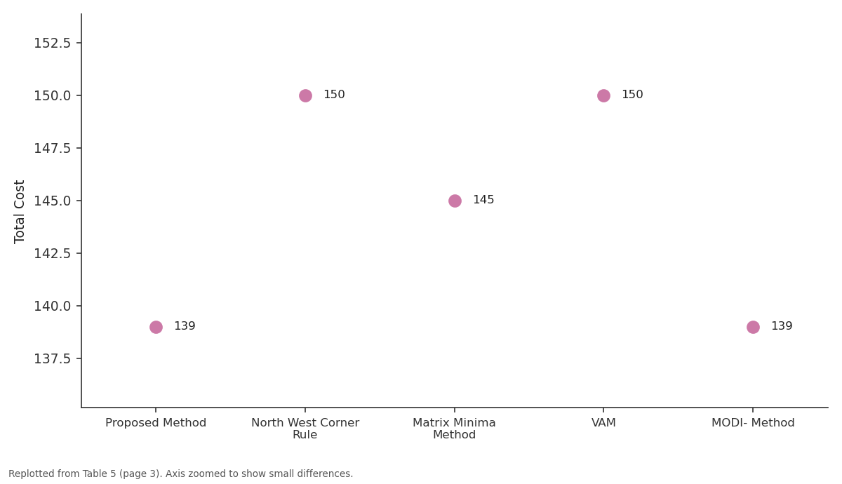
Example 3.1: Proposed Method vs North West Corner Rule vs Matrix Minima Method vs VAM vs MODI- Method
Replotted from Table 5 (page 3) of the original paper. Every bar is the paper's own table value.
View source evidence ↗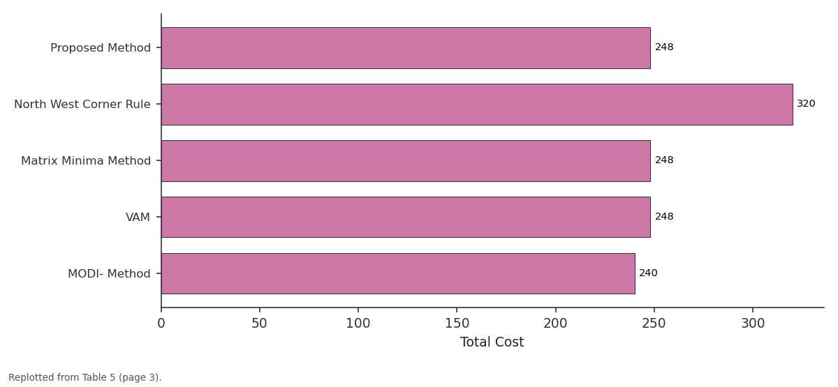
Example 3.2: Proposed Method vs North West Corner Rule vs Matrix Minima Method vs VAM vs MODI- Method
Replotted from Table 5 (page 3) of the original paper. Every bar is the paper's own table value.
View source evidence ↗Figures & tables
From the original paper Table 1
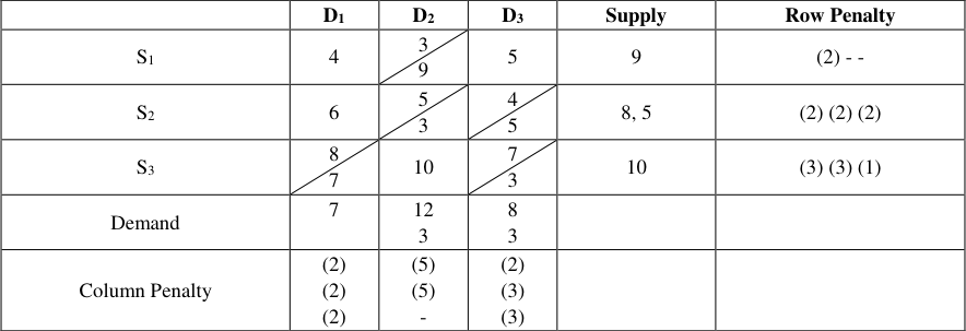 Table 2
 Table 3
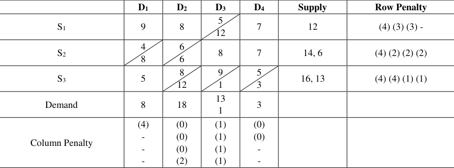 Table 4
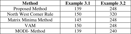 Table 5
Introduction
A transportation problem is one of the earliest and most important applications of linear programming problem. Which can be applied for different sources f supply to different destination of demand in such a way that the total transportation cost should be minimized. Usually, the initial basic feasible solution of any transportation problem is obtained by using well known methods such as North West Corner Method or Least-Cost Method or Vogel’s Approximation Method, and then finally the optimality of te given transportation problem is checked by MODI. Afterwards many researchers provide many methods to solve transportation problem.
Some of the important related works the current research has deal with are: ‘Modified Vogel’s Approximation Method for Unbalance Transportation Problem’, [2] by N. Balakrishnan. ‘An Improved Vogel’s Approximation method [3] by Serder Korukogu and Serkan Balli., ‘A new approach for find an Optimal Solution for Transportation Problems’, [6] by Sudhakar VJ et.al In last few year S. Rekha, et al. [5], M. Wali Ullah et al [1] and S.M.
Abul Kalam [4] developed the method is very helpful as having less computations and also required the short time of period for getting the optimal solution. In this paper we introduce Method for solving transportation problem which is very simple, easy to understand and helpful for decision making and it gives minimum solution of transportation problem. The method developed here ensures a solution which is very closer to the optimal solution. 2. Algorithm of Proposed Method Step 1: Examine whether the transportation problem is balanced or not.
If it is balanced then go to next step. Step 2: Find the difference between maximum and minimum in each row which is called as row penalty and difference between maximum and next maximum in each column which is called as column penalty and write it in the side and bottom. Step 3: From that select the maximum value. From the selected row/column we need to allocate the minimum of supply/demand in the minimum element of the row or column.
Eliminate by deleting the columns or rows corresponding to where the supply or demand is satisfied. Maths 2017; 2(6): 43-45 Sarla Raigar Research Scholar, Department of Mathematics, Govt. M.V.M. Bhopal, Madhya Pradesh, India Sushma Duraphe Department of Mathematics, Govt.
M.V.M. Bhopal, Madhya Pradesh, India Geeta Modi Department of Mathematics, Govt. M.V.M. Bhopal, Madhya Pradesh, India Correspondence Sarla Raigar Research Scholar, Department of Mathematics, Govt.
M.V.M. Bhopal, Madhya Pradesh, India Step 6: Now total minimum cost is calculated as sum of the product of cost and corresponding allocate value of supply/demand. 3. Numerical Example Example 3.1. Illustrate Step 4: If obtained condition in step 3 is contrary, that is if there is tie in maximum value select that value which has least element.
If there is tie in the least element then allocate the least element which has minimum supply/ demand. Step 5: Repeating the step 2 to step 4 until satisfaction of all the supply and demand is met. Table 1 D1 D2 D3 Supply S1 4 3 5 9 S2 6 5 4 8 S3 8 10 7 10 Demand 7 12 8 Solution: since Σai = Σbj = 27 The given transportation problem is balanced; therefore exist a basic feasible solution to Proposed Method problem. Table 2 D1 D2 D3 Supply Row Penalty S1 4 3 9 5 9 (2) - - S2 6 5 3 4 5 8, 5 (2) (2) (2) S3 8 7 10 7 3 10 (3) (3) (1) 12 Demand 7 3 8 3 Column Penalty (5) (5) (2) (2) (2) - (2) (3) (3) The transportation cost is: Z = 3*9 + 5*3 + 4*5 + 8*7 + 7*3 = 139/- Example 3.2.
| — | D1 | D2 | D3 | Supply |
|---|---|---|---|---|
| S1 | 4 | 3 | 5 | 9 |
| S2 | 6 | 5 | 4 | 8 |
| S3 | 8 | 10 | 7 | 10 |
| Demand | 7 | 12 | 8 |
Table text extracted from the original PDF; superscript letters are shown inline. The original table image is below.
View original table image
Illustrate Table 3 D1 D2 D3 D4 Supply S1 9 8 5 7 12 S2 4 6 8 7 14 S3 5 8 9 5 16 Demand 8 18 13 3 Solution : since Σai = Σbj = 42 The given transportation problem is balanced; therefore exist a basic feasible solution to Proposed Method problem. Table 4 D1 D2 D3 D4 Supply Row Penalty S1 9 8 5 12 7 12 (4) (3) (3) - S2 4 8 6 6 8 7 14, 6 (4) (2) (2) (2) S3 5 8 12 9 1 5 3 16, 13 (4) (4) (1) (1) Demand 8 18 13 1 3 (4) (0) (0) Column Penalty - - - (0) (0) (0) (2) (1) (1) (1) (1) - - The transportation cost is Z = 5*12 + 4*8 + 6*6 + 8*12 + 9*1 + 5*3 = 248/- Comparison of the numerical results Comparison of the numerical results which are obtain from the example is shown in the following table Table 5 Method Example 3.1 Example 3.2 Proposed Method 139 248 North West Corner Rule 150 320 Matrix Minima Method 145 248 VAM 150 248 MODI- Method 139 240
| Method | Example 3.1 | Example 3.2 |
|---|---|---|
| Proposed Method | 139 | 248 |
| North West Corner Rule | 150 | 320 |
| Matrix Minima Method | 145 | 248 |
| VAM | 150 | 248 |
| MODI- Method | 139 | 240 |
Table text extracted from the original PDF; superscript letters are shown inline. The original table image is below.
View original table image
| — | D1 | D2 | D3 | D4 | Supply |
|---|---|---|---|---|---|
| S1 | 9 | 8 | 5 | 7 | 12 |
| S2 | 4 | 6 | 8 | 7 | 14 |
| S3 | 5 | 8 | 9 | 5 | 16 |
| Demand | 8 | 18 | 13 | 3 |
Table text extracted from the original PDF; superscript letters are shown inline. The original table image is below.
View original table image
Conclusion
The proposed method is an attractive method which is very simple, easy to understand and gives result exactly or even lesser to VAM method. All necessary qualities of being time efficient, easy applicability etc., forms the core of being implemented successfully.
References
6 in the original paper- Wali Ullah M, Alhaz Uddin M, Rijwana Kawser. ‘A Modified Vogel’s Approximation Method for Obtaining a Good Primal Solution of Transpotation Problem, Annals of Pure ans Applied Mathematics. 2016; 11(1):63-71.
- Balakrishnan N. ‘Mdified Vogel’s Approximation Method for Unbalance Transportation Problem’, Applied Mathematics Letters. 1990; 3(2):9-11.
- Serder Korukogu, Serkan Balli. ‘An Improved Vogel’s Approximation method for the transportation problem’, Association for Scientific Research, Mathematical and Computation. 2011; 16(2):370-381.
- Abul Kalam SM, Azad Md, Belle Hossain. A New Method for Solving Transportation Problems Considering Average Penalty IOSR Journal of Mathematics. 2017; 13(1):40-43
- Rekha S, Srividhya B, Vidya S Transportation Cost Minimization: Max Min Penalty Approach IOSR Journal of Mathematics. 2014; 10(2):6-8.
- Sudhakar VJ, Arunnsankar N, Karpagam T. A new approach for find an Optimal Solution for Transportation Problems, European Journal of Scientific Research. 2012; 68(2):254-257.
Cited by 2
From OpenAlex, OpenCitations and reference lists read by Scinovex
- A Comprehensive Method for Arriving at Initial Feasible Solution for Optimization Problems in Engineering with Illustrative Examples ↗
Et. al. Chandrasekhar Putcha · Türk bilgisayar ve matematik eğitimi dergisi · 2021
Two methods have been used extensively for arriving at initial basic feasible solution (IBF). One of them is Northwest corner rule and the other on is Russell method (Hillier & Lieberman, 2005.) Both methods have drawbacks. The IBF obtained is either far from optimal solution or does not have adequate number of entries to initiate transportation simplex algorithm. The Northwest…
❝ 3PDF - Analysis of Transportation Method in Optimization of Distribution Cost Using Stepping Stone Method and Modified Distribution ↗
Annisa Annisa, Mardiningsih Mardiningsih · Journal of Mathematics Technology and Education. · 2021
This study aims to examine each method to show the characteristics, advantages and disadvantages of the transportation problem solving method. Vogel Approximation Method (VAM) is an initial solution method that is better than other methods and generally produces an initial solution that is close to the optimum result. In this study the Stepping Stone and Modified Distribution methods produce the…
❝ 1PDF