
Research article · 2018 · Full text
International Journal of Statistics and Applied MathematicsParameter estimation for the Exponentiated Weibull distribution: Comparative study
Volume 3(2) · Pages 111–117
Research areasStatistical Distribution Estimation and Applications
Abstract
Author-writtenFor the estimation of probability distribution parameters, Haktanir (1997) [4] introduced the method of self-determined probability weighted moments as a refinement on the original method of probability weighted moments defined by Greenwood et al (1979) [2]. In this study, simulation experiments were conducted to investigate the performance of the self- determined probability weighted moments method versus the performances of the methods of maximum likelihood and moments in estimating the parameters of the Exponentiated Weibull distribution.
Summary
Source-checkedPlain-language reading of the full paper, prepared with AI and checked against the text. Each point links to the authors' own words.
Why it matters
- Maximum likelihood (ML) and method of moments (MM) are common parameter estimation techniques, with ML relying on large sample theory and MM valued for its simplicity. View evidence ↗
- Probability weighted moments (PWM) were developed as an alternative to ML because PWM performs better when working with small sample sizes. View evidence ↗
- The self-determined probability weighted moments (SDPWM) method refines PWM by allowing for the detection of appropriate distributions and the direct consideration of outliers. View evidence ↗
The question
- The study aims to evaluate the efficiency of the SDPWM method for estimating Exponentiated Weibull distribution parameters compared to ML and MM methods. View evidence ↗
What they did
- The researchers used Mathcad version 14.0 to implement estimation algorithms and solve the required non-linear equations through iterative procedures. View evidence ↗
- The performance of the estimators was compared based on two primary metrics: bias and mean square error (MSE). View evidence ↗
What they found
- The method of moments (MM) was found to be the least effective method, exhibiting the highest bias and MSE. View evidence ↗
What it means
- The authors conclude that SDPWM is the most effective method regarding bias and MSE, particularly when dealing with small sample sizes. View evidence ↗
Visual summary
3 visualsIllustrations explain the paper; charts are replotted from the paper's own table values.
Comparison Framework
AI-generated conceptual illustration (A set of scattered data points on a coordinate plane). It explains the idea and does not show study data.
View source evidence ↗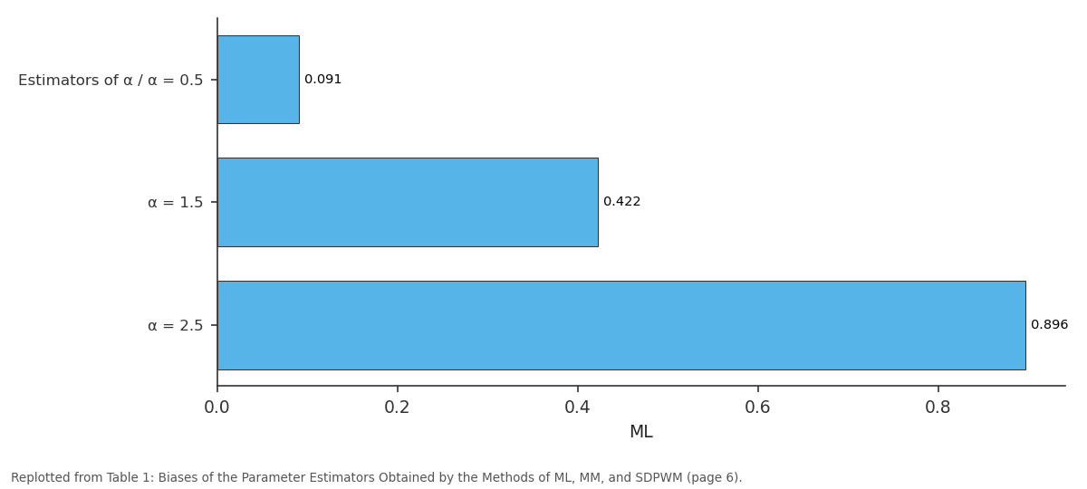
ML: Estimators of α / α =... vs α = 1.5 vs α = 2.5
Replotted from Table 1 (page 6) of the original paper. Every bar is the paper's own table value.
View source evidence ↗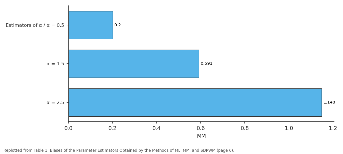
MM: Estimators of α / α =... vs α = 1.5 vs α = 2.5
Replotted from Table 1 (page 6) of the original paper. Every bar is the paper's own table value.
View source evidence ↗Figures & tables
From the original paper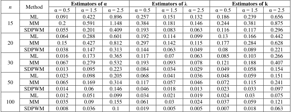 Table 1
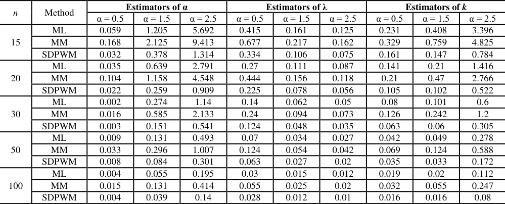 Table 2
Introduction
In most statistical studies the population parameters are unknown and must be estimated from a sample. The maximum likelihood (ML) method is an important method of estimation, whose justification is based on large sample theory; whereas the method of moments (MM) is mostly used because of its relative ease of application. Since the ML method does not always work well in small samples, other methods of estimation were developed as alternatives. Among these is the probability weighted moments (PWM) method which was devised by Greenwood et al (1979) [2] . This method works very well with small samples. In addition, it was found to posses some desirable statistical properties, it is also computationally simple and robust. Another method of estimation is the method of self-determined probability weighted moments (SDPWM) which was proposed by Haktanir (1997) [4] as a refinement on the original method of PWM. It has many advantages over the method of PWM, such as the ability to directly consider outliers and the ability to detect whether a particular distribution is appropriate for describing a sample. The Exponentiated Weibull distribution was introduced by Mudholkar and Srivastava (1993) as an extension of the Weibull distribution by adding a second shape parameter. The cumulative distribution function for the Exponentiated Weibull distribution is:
, then the Exponentiated Weibull distribution coincides with the Weibull distribution with a scale parameter . Also, when the shape parameter k=1 then it will be the Exponentiated exponential distribution.
The main aim of this paper is to study the efficiency of the SDPWM method in estimating the parameters of the Exponentiated Weibull distribution through comparing it with the more conventional methods of estimation, which are the methods of ML and MM. In the three methods of estimation, determination of parameter estimates requires solving non-linear equations. Therefore, all estimation algorithms are implemented using the Mathcad (version 14.0) software, which contains iterative procedures that are useful for solving the aforementioned non-linear equations. The organization of this article is as follows. A theoretical overview of the method of SDPWM is provided in section 2. In section 3, the SDPWM estimation of the Exponentiated Weibull parameters is discussed. Then, sections 4 and 5 explain the estimation of the Exponentiated Weibull parameters by the methods of ML and MM, respectively. Section 6 contains simulation results and discussions. Finally, conclusions are included in section 7. Results tables are included in the appendix.
Overview
The method of self-determined probability weighted moments was proposed as a modification of the original method of PWM. The probability weighted moments of a random variable X with cumulative distribution function
The two PWM sets, s and r , are linear combinations of each other. Therefore, any one of them can be used; whichever is possible; for parameter estimation without loss of generality.
To estimate the parameters of a distribution, a sample estimator of s or r is needed. Landwehr et al (1979a) [7] introduced unbiased estimators of from the distribution F . They are given by:
probabilities, respectively; and
is the ith observation in the ordered sample. These estimates are not based on the assumed distribution, but are based solely on the position of
within the ordered sample.
The method of SDPWM deviates from the method of PWM in that it is assumed that the ordered sample follows a particular distribution. Accordingly, the non-exceedance probabilities are assigned using the corresponding cumulative distribution function of the assumed distribution. Therefore, the SDPWM sample estimators s ~ and r ~ for s and r , respectively, are defined as follows:
Where F is the distribution function of a given distribution;
are the unknown parameters of this distribution; and
Self-Determined Probability Weighted Moments Estimators
For the Exponentiated Weibull distribution, it is more convenient to work with the PWM of the form r which is given by:
Since the Exponentiated Weibull distribution is a three-parameter distribution, then only the first three PWM; 0 , 1 and 2 are needed. They are given as follows:
In the original method of PWM, the population PWMs ( 0 , 1 , 2 ) are replaced with the PWM sample estimators calculated as in equation (2.5). The procedure of SDPWM estimation of the Exponentiated Weibull parameters is the same as the procedure of PWM estimation. The difference is that in the case of SDPWM estimation, the population PWMs ( 0
3) and (3.4) will be replaced by the SDPWM sample estimators, 0 , 1 and 2 , where:
Therefore, the SDPWM parameter estimators,
, can be obtained by replacing the population
2), (3.3) and (3.4) by the SDPWM sample estimators ( 0 , 1 , 2 ). Then, this will make three new equations that are:
Which can be solved simultaneously by numerical simulation to obtain the estimates.
Maximum Likelihood Estimators
The method of maximum likelihood is one of the best known, most widely used, and most important of the methods of estimation.
In this section, the procedure of the ML estimation of the parameters of the Exponentiated Weibull distribution is discussed as follows.
, from the Exponentiated Weibull distribution; the likelihood function ( , k , ) L is given by: International Journal of Statistics and Applied Mathematics
Then the ML estimators; ˆML , ˆML k and ˆML ;can be obtained by simultaneously solving the following three equations by numerical simulation:
Moments Estimators
The method of moments (MM) is one of the oldest methods used for generating estimates for the unknown parameters from sample data. was first proposed by Pearson (1894) and was used extensively for many years. In this section, the procedure of the MM estimation of the parameters of the Exponentiated Weibull distribution is illustrated as follows.
Since there are three parameters to be estimated then the first three moments; 1 , 2 and 3 ; are needed. They are given by: ). This will yield the three following equations:
The three equations (5.7), (5.8) and (5.9) can be solved simultaneously by numerical simulations to obtain the moment estimators ˆMM , ˆMM k and ˆMM .
Comparative Study
Since it is difficult to compare the performances of the different estimators (described in the previous sections) theoretically, extensive computer simulations are performed to conduct this comparison. The properties of the different estimators are compared mainly in terms of bias and mean square error (MSE), for different sample sizes and for different values of the shape parameter . The simulation experiments are performed using the Mathcad (version 14.0) software. Different sample sizes are considered through the experiments that are n 15, 20, 30, 50 and 100. In addition, different values for the shape parameter are considered, which are 0.5, 1.5 and 2.5 with the two parameters k and taken to be 1 in all the experiments. For each combination of the sample size and -value the experiment will be repeated 10000 times. In each experiment, the estimates of , k and will be obtained by the different methods described in the previous sections. The biases and MSEs for the different estimators will be reported from these experiments. The algorithm for obtaining the different estimates by the different methods of estimation can be described in details in the following steps:
Step (1): Generate a random sample of size n,
, from the Exponentiated Weibull distribution. This can be achieved by firstly generating a random sample from the uniform (0,1) distribution,
. Then the uniform random numbers can be transformed into Exponentiated Weibull random numbers using the following transformation:
Step (2): Sort the random sample . Note that this step is required for SDPWM estimation. The ML and MM methods do not require the sample to be ordered for parameter estimation. The biases and MSEs of the different estimators are reported in tables ( 1) and (2), respectively. From these tables many observations can be made on the performance of the methods of SDPWM versus the methods of ML and MM. These observations are summarized as follows:
(1) It is observed that the biases and MSEs of the different estimators depend on the value of the shape parameter . For all the methods considered as increases the biases and MSEs of the estimators of and k increase. On the other hand, the biases and MSEs of the estimators of decrease as increases for all the methods. (2) For all the cases considered the biases and MSEs of the different estimators of , k and decrease as the sample size increases. This indicates that all the methods provide consistent estimators for , k and . (3) Comparing the biases of the different estimators of , k and , it is clear that the method of SDPWM yields the minimum bias in almost all the cases considered. (4) Considering the MSEs of the different estimators of , it is clear from table (2) that the SDPWM estimator has the minimum MSE in almost all of the cases considered for estimating . On the other hand, the MM method is the worst in terms of bias and MSE.
Conclusions
The comparative study revealed that the SDPWM works the best in almost all the cases considered with respect to MSE and Bias, especially for small sample sizes. The of the MM method is the worst in terms of bias and MSE. In addition, all the methods considered have provided consistent estimators for , k and .
Appendix
Appendix
Figures and tables from the paper
| n | Method | Estimators of α | — | — | Estimators of λ | — | — | Estimators of k | — | — |
|---|---|---|---|---|---|---|---|---|---|---|
| α = 0.5 | α = 1.5 | α = 2.5 | α = 0.5 | α = 1.5 | α = 2.5 | α = 0.5 | α = 1.5 | α = 2.5 | ||
| 15 | ML | 0.091 | 0.422 | 0.896 | 0.257 | 0.151 | 0.132 | 0.186 | 0.239 | 0.656 |
| MM | 0.2 | 0.591 | 1.148 | 0.384 | 0.181 | 0.146 | 0.244 | 0.381 | 0.875 | |
| SDPWM | 0.055 | 0.201 | 0.409 | 0.193 | 0.083 | 0.063 | 0.116 | 0.117 | 0.296 | |
| 20 | ML | 0.064 | 0.288 | 0.601 | 0.192 | 0.114 | 0.099 | 0.13 | 0.166 | 0.442 |
| MM | 0.15 | 0.427 | 0.812 | 0.297 | 0.142 | 0.115 | 0.177 | 0.284 | 0.628 | |
| SDPWM | 0.038 | 0.147 | 0.313 | 0.144 | 0.063 | 0.049 | 0.08 | 0.089 | 0.221 | |
| 30 | ML | 0.016 | 0.173 | 0.365 | 0.117 | 0.07 | 0.063 | 0.085 | 0.103 | 0.266 |
| MM | 0.067 | 0.279 | 0.532 | 0.193 | 0.093 | 0.078 | 0.121 | 0.188 | 0.407 | |
| SDPWM | 0.013 | 0.095 | 0.223 | 0.084 | 0.034 | 0.029 | 0.049 | 0.058 | 0.154 | |
| 50 | ML | 0.023 | 0.098 | 0.205 | 0.068 | 0.041 | 0.036 | 0.048 | 0.059 | 0.151 |
| MM | 0.065 | 0.169 | 0.314 | 0.117 | 0.057 | 0.046 | 0.072 | 0.115 | 0.241 | |
| SDPWM | 0.014 | 0.06 | 0.146 | 0.046 | 0.018 | 0.013 | 0.023 | 0.033 | 0.097 | |
| 100 | ML | 0.012 | 0.051 | 0.099 | 0.034 | 0.021 | 0.019 | 0.024 | 0.03 | 0.075 |
| MM | 0.035 | 0.09 | 0.155 | 0.061 | 0.03 | 0.024 | 0.037 | 0.059 | 0.121 | |
| SDPWM | 0.008 | 0.036 | 0.1 | 0.019 | 0.005 | 0.005 | 0.007 | 0.018 | 0.063 |
Table text extracted from the original PDF; superscript letters are shown inline. The original table image is below.
View original table image
| n | Method | Estimators of α | — | — | Estimators of λ | — | — | Estimators of k | — | — |
|---|---|---|---|---|---|---|---|---|---|---|
| α = 0.5 | α = 1.5 | α = 2.5 | α = 0.5 | α = 1.5 | α = 2.5 | α = 0.5 | α = 1.5 | α = 2.5 | ||
| 15 | ML | 0.059 | 1.205 | 5.692 | 0.415 | 0.161 | 0.125 | 0.231 | 0.408 | 3.396 |
| MM | 0.168 | 2.125 | 9.413 | 0.677 | 0.217 | 0.162 | 0.329 | 0.759 | 4.825 | |
| SDPWM | 0.032 | 0.378 | 1.314 | 0.334 | 0.106 | 0.075 | 0.161 | 0.147 | 0.784 | |
| 20 | ML | 0.035 | 0.639 | 2.791 | 0.27 | 0.111 | 0.087 | 0.141 | 0.21 | 1.416 |
| MM | 0.104 | 1.158 | 4.548 | 0.444 | 0.156 | 0.118 | 0.21 | 0.47 | 2.766 | |
| SDPWM | 0.022 | 0.259 | 0.909 | 0.225 | 0.078 | 0.056 | 0.105 | 0.102 | 0.522 | |
| 30 | ML | 0.002 | 0.274 | 1.14 | 0.14 | 0.062 | 0.05 | 0.08 | 0.101 | 0.6 |
| MM | 0.016 | 0.585 | 2.133 | 0.24 | 0.094 | 0.073 | 0.126 | 0.242 | 1.2 | |
| SDPWM | 0.003 | 0.151 | 0.541 | 0.124 | 0.048 | 0.035 | 0.063 | 0.06 | 0.305 | |
| 50 | ML | 0.009 | 0.131 | 0.493 | 0.07 | 0.034 | 0.027 | 0.042 | 0.049 | 0.278 |
| MM | 0.033 | 0.296 | 1.007 | 0.124 | 0.054 | 0.042 | 0.069 | 0.124 | 0.588 | |
| SDPWM | 0.008 | 0.084 | 0.301 | 0.063 | 0.027 | 0.02 | 0.035 | 0.033 | 0.172 | |
| 100 | ML | 0.004 | 0.055 | 0.195 | 0.03 | 0.015 | 0.012 | 0.019 | 0.02 | 0.112 |
| MM | 0.015 | 0.131 | 0.414 | 0.055 | 0.025 | 0.02 | 0.032 | 0.055 | 0.247 | |
| SDPWM | 0.004 | 0.039 | 0.14 | 0.028 | 0.012 | 0.01 | 0.016 | 0.016 | 0.08 |
Table text extracted from the original PDF; superscript letters are shown inline. The original table image is below.
View original table image
References
10 in the original paper- Bartolucci AA, Singh KP, Bartolucci AD, Bae S. Applying medical survival data to estimate the three-parameter Weibull distribution by the method of probability-weighted moments, Mathematics and computers in simulation, 1999; 48(4):385-392.
- Greenwood JA, Landwehr JM, Matalas NC, Wallis JR. Probability weighted moments: definition and relation to parameters of several distributions expressible in inverse form, Water Resources Research, 1979; 15(5):1049-1054.
- Gupta RD, Kundu D. Discriminating between Weibull and generalized exponential distribution, Computational statistics and data analysis, 2003; 43:179-196.
- Haktanir T. Self-determined probability-weighted moments method and its application to various distributions, Journal of Hydrology, 1997; 194(1-4):180-200.
- Hosking JRM, Wallis JR, Wood EF. Estimation of the Generalized Extreme-Value Distribution by the Method of Probability weighted moments, Technometrics, 1985; 27(3):251-261.
- Hosking JRM, Wallis JR. Parameter and Quantile Estimation for the Generalized Pareto Distribution, Technometrics, 1987; 29(3):339-349.
- Pearson K. Contributions to the Mathematical Theory of Evolution. II Skew Variations in Homogeneous Material, Philosophical Transactions of the Royal Society of London, Series A, 1894; 186:343-414.
- Savage GT, Whalen TM, Jeong GD. Application of the self-determined probability-weighted moment method to extreme wind speed estimation, Proceedings of the Americas Conference on Wind Engineering, June 4-6, 2001, Clemson University, Clemson, SC., 2001.
- Song D, Ding J. The application of probability weighted moments in estimating the parameters of the Pearson Type Three distribution, Journal of Hydrology, 1988; 101:47-61.
- Whalen TM, Savage GT, Jeong GD. The Method of Self-Determined Probability Weighted Moments Revisited, Journal of Hydrology, 2002; 268(1-4):177-191.