
Research article · 2018 · Full text
International Journal of Statistics and Applied MathematicsA hybrid group acceptance sampling plan for lifetimes based on transmuted exponential distribution
Volume 3(2) · Pages 268–273
Research areasStatistical Distribution Estimation and Applications
Abstract
Author-writtenIn this paper, we have proposed a hybrid group acceptance sampling plan (HGASP) for a truncated life test when the lifetime of an item follows transmuted exponential distribution. The minimum number of testers and acceptance number are determined when the consumer’s risk and the test termination time and group size are specified. The operating characteristic values according to various quality levels are obtained. The minimum ratios of the true median and specified median for the given producer’s risk are also determined. The results are discussed through an example, comparative study of proposed sampling plan with existing sampling plan are explained.
Summary
Source-checkedPlain-language reading of the full paper, prepared with AI and checked against the text. Each point links to the authors' own words.
Why it matters
- Statistical quality control is critical for industrial success because product quality is a primary factor in a highly competitive global market. View evidence ↗
- Acceptance sampling plans provide a balanced approach between performing a full inspection of all items and performing no inspection. View evidence ↗
- Using testers that can hold multiple items simultaneously is common in practice to reduce both the cost and the time required for testing. View evidence ↗
The question
- The research aims to propose a hybrid group acceptance sampling plan (HGASP) specifically for truncated life tests where item lifetimes follow a transmuted exponential distribution. View evidence ↗
What they did
- The plan involves selecting a number of testers (r) and assigning them to predefined groups (g), resulting in a total sample size of n = rg. View evidence ↗
- The test termination time (t0) is defined as a multiple of the specified mean life (𝜇0), using a termination ratio 'a'. View evidence ↗
What they found
- For a fixed number of groups, increasing the test termination time multiplier (a) generally reduces the minimum number of testers (r) required. View evidence ↗
- With parameters 𝛽=0.25, g=4, c=2, and a=0.7, the required testers are r=4; the producer's risk decreases from 0.2842 to 0.0195 as the true mean lifetime increases from 2 to 6 times the specified mean. View evidence ↗
- To achieve a producer's risk of 𝛼=0.05 with 𝛽=0.25, r=4, g=4, c=2, and a=0.7, the true mean must be 4.21 times the specified mean. View evidence ↗
What it means
- The authors conclude that their proposed HGASP is more beneficial and economical than existing plans regarding labor, cost, truncation time, and sample size. View evidence ↗
Visual summary
2 visualsIllustrations explain the paper; charts are replotted from the paper's own table values.

HGASP Workflow
AI-generated conceptual illustration (Electronic components on a testing circuit board). It explains the idea and does not show study data.
View source evidence ↗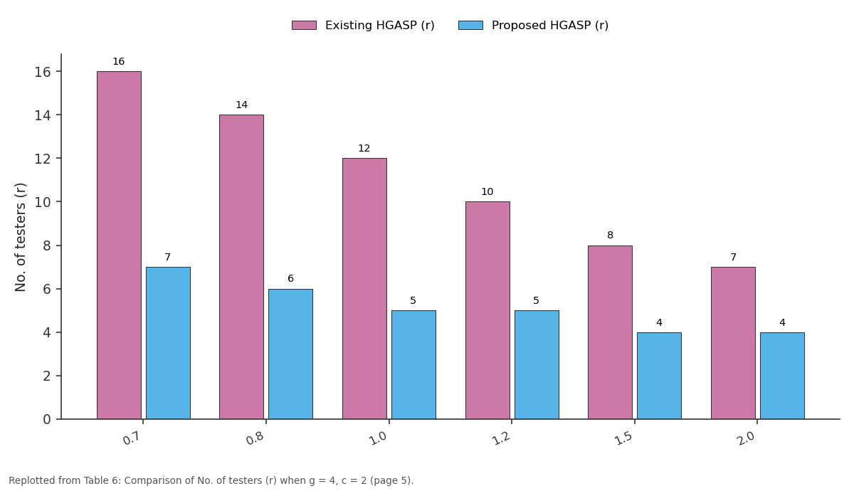
Existing HGASP (r) and Proposed HGASP (r): 0.7 vs 0.8 vs 1.0 vs 1.2 vs 1.5
Replotted from Table 6 (page 5) of the original paper. Every bar is the paper's own table value.
View source evidence ↗Figures & tables
From the original paper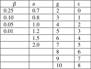 Table 1
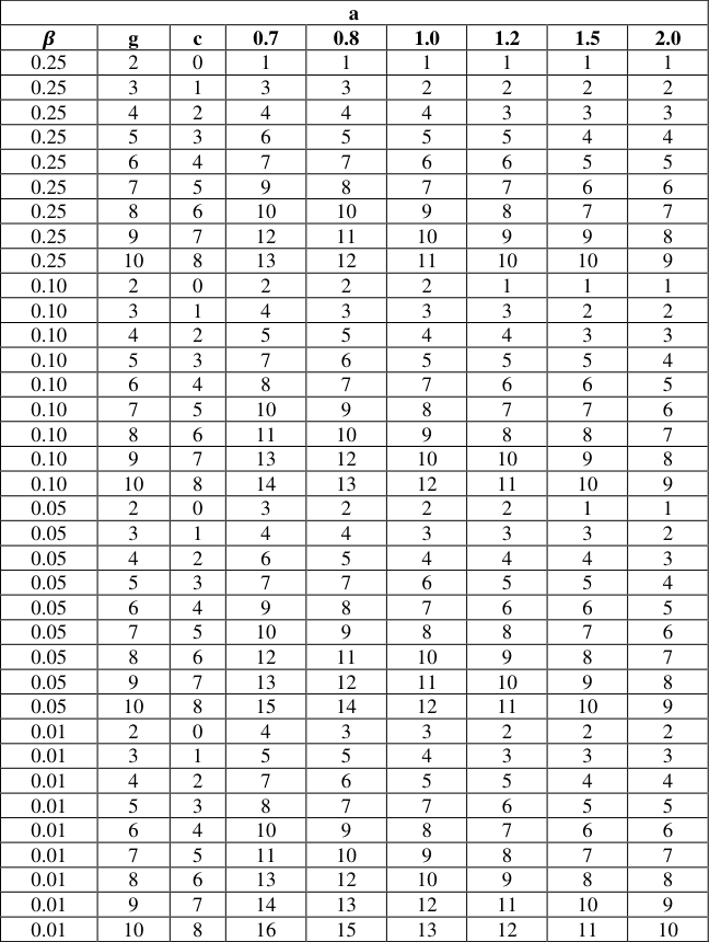 Table 2
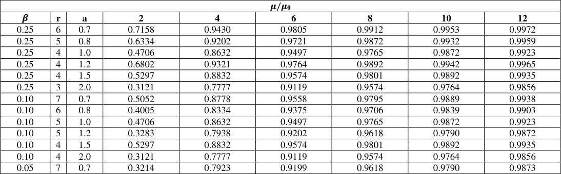 Table 3
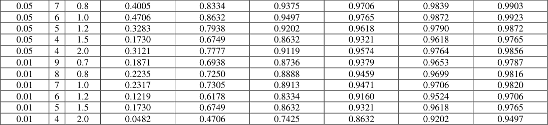 Table 4
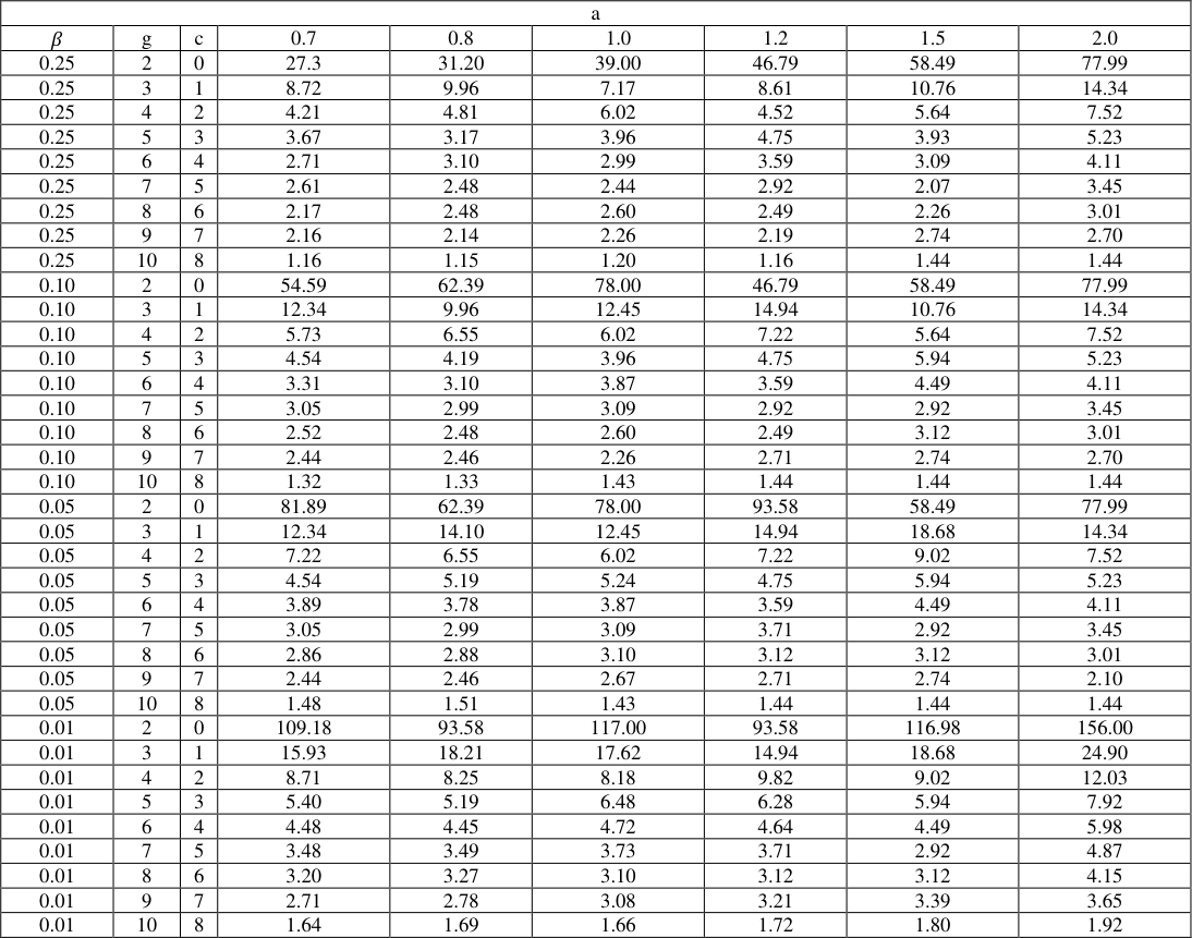 Table 4
 Table 5
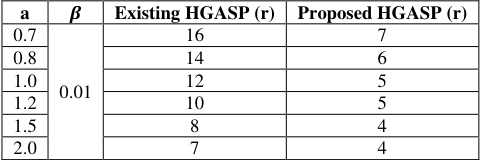 Table 6
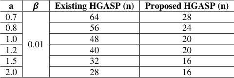 Table 7
Introduction
Today quality of products definitely plays one of the most important roles due to highly competitive global market, for any industry. For this reason, statistical quality control plays a significant role for the success or failure of an industry. It is very clear that in many situations it may not be possible to perform hundred percent inspection. On the other hand, if nothing is tested, desired quality cannot be assured. For this purpose, acceptance sampling plans plays an essential tool in statistical quality control. Acceptance sampling plan is a " middle path" between hundred percent inspection and no inspection at all. The acceptance sampling is concerned with accepting or rejecting a submitted lot of products on the basis of the quality of the products inspected in a sample taken from the lot. An acceptance sampling plan is a scheme that establishes the minimum sample size to be used for testing. This becomes particularly important if the quality of product is defined by its lifetime. Often, it is implicitly assumed when designing a sampling plan that only a single item is put in a tester. However, in practice testers accommodating a multiplier number of items at a time are used because testing time and cost can be saved by testing items simultaneously. The item in a group is called the group size. An acceptance sampling plan based on such groups of items is called a Group Acceptance Sampling Plan (GASP). The method of determining the minimum number of testers for a predetermined number of groups is called as Hybrid Group Acceptance Sampling Plan (HGASP). If the HGASP is used in conjunction with truncated life test assuming that the life time of product follows a certain probability distribution. For such a type of test, the determination of the sample size is equivalent to determine the number of testers. This type of testers is frequently used in sudden death testing. Some ordinary acceptance sampling plans are discussed by Aslam, Kundu and Ahmad [11] for generalized exponential distribution, Al-omari and Zamande [2] studied double acceptance sampling plan for time truncated life tests based on transmuted generalized inverse weibull distribution, Abdur Razzaque Mughal [1] presented a hybrid economic group acceptance sampling plan for exponential lifetime distribution, Srinivasa Rao [9] developed a hybrid group acceptance sampling plans for lifetimes based on generalized exponential distribution, Subba Rao, Naga Durgamamba, Kantam [12] derived hybrid group acceptance sampling plan based on size biased lomax model, JafferHussain, AbdurRazzaque Mughal, Muhammad Khalid Pervaiz and Usman Ali [5] discussed a hybrid group acceptance sampling plan for lifetimes having generalized pareto distribution.
The purpose of this research is to propose a HGASP based on truncated life tests when the lifetime of a product follows the transmuted exponential distribution. Let T be a lifetime that is distributed according to transmuted exponential distribution with two parameters |𝜆 ≤ 1|, 𝜃>0. The probability density function (pdf) and cumulative density function (cdf) of the transmuted exponential distribution respectively, are given by:
Where 𝜃and 𝜆 are scale and shape parameters respectively.
The mean of this distribution for 𝜆=1 is given by 𝜇 = 𝜃 ( 2-𝜆 2 ) = 0.5 𝜃. For more information about the transmuted exponential distribution, we refer the interested reader to [7] .
The suggested hybrid group acceptance sampling plan is given in section 2. The operating characteristic function are presented in section 3. Producer's risk is given in section 4. Description of tables and examples are provided for an illustration in section 5. The comparative study is presented in section 6. The conclusion is given in section 7.
The hybrid group acceptance sampling plan
Let 𝜇 denotes the true mean life of a product and 𝜇0 represents the specified mean life of an item, under the assumption that the lifetime of an item follows transmuted exponential distribution. A product is considered as good and accepted for consumer's use if the sample information supports the hypothesis H0: 𝜇 ≥ 𝜇0. On the other hand, the lot of the product is rejected. In acceptance sampling schemes, this hypothesis is tested based on the number of failures from a sample in a prefixed time. If the number of failures exceeds the acceptance number c we reject the lot. We will accept the lot if there is enough evidence that 𝜇 ≥ 𝜇0 at certain level of consumer's risk. Otherwise, we reject the lot. Let us prepare the following HGASP based on the truncated life test. Select the number of testers, r and assign the r items to each predefined groups, g, the required sample size for a lot is n = rg. Prefix the acceptance number, c for each group and the experiment time t0. Accept the lot if atmost c failures occur in each of all groups. Terminate the experiment if more than c failures occur in any group and reject the lot. We are interested in determining the number of testers, r, required for transmuted exponential distribution and various values of acceptance number, c, whereas the number of groups, g and the termination time t0 are assumed to be specified. Since it is convenient to set the termination time as a multiple of the specified value 𝜇0 of the mean, we will consider t0 = a 𝜇0 for a given constant, 'a' (termination ratio). The probability (𝛼) of rejecting a good lot when the sample is bad one, which is called the producer's risk whereas the probability (𝛽) of accepting a bad lot when the sample is good one, which is known as the consumer's risk. The parameter value r of the proposed sampling plan is determined for ensuring the consumer's risk. Often, the consumer's risk will be 𝛽 = 1-p * . We will determine the number of testers r in the proposed sampling plan so that the consumer's risk does not exceed a given value 𝛽. If the lot size is large enough, we can use the binomial distribution to develop the HGASP.
According to the HGASP, the lot of products is accepted only if there are atmost 'c' failures observed in each of the 'g' groups. The HGASP is characterized by the three parameters. The lot acceptance probability is:
Where, p is the probability that an item in a tester fails before the termination time t0 = a 𝜇0. The probability p for the transmuted exponential distribution with 𝜆=1 is given by:
The minimum number of testers required can be determined by considering the consumer's risk when the true mean life equals the specified mean life (𝜇 = 𝜇0) through the following inequality:
Where, P0 is the failure probability at (𝜇 = 𝜇0) and it is given by:
Operating Characteristics
The probability of acceptance can be regarded as a function of the deviation of specified mean from the true mean. This function is called operating characteristics (OC) function of the sampling plan. Once the minimum number of testers is obtained, one may be interested to find the probability of acceptance of a lot when the quality (or reliability) of the product is good enough. As mentioned earlier, the product is considered to be good if 𝜇 > 𝜇0 (or) 𝜇/𝜇0. For 𝜆=1 the probabilities of acceptance are displayed in Table 3. Based on equation (3) for various values of the mean ratios 𝜇/𝜇0, producer's risk 𝛽 and the time multiplier 'a' that are given in Table 1. From Table 3, we see that OC values increase more quickly as the mean ratio increases. For example, when 𝛽 = 0.25, g=4, c=2 and a=0.7, the number of testers required is r=4. However, if the true mean lifetime is twice the specified mean lifetime (𝜇/𝜇0 =2) the producer's risk is approximately 𝛼 = 1-0.7158 = 0.2842, while 𝛼 = 0.0195 when the true value of mean is 6 times the specified one.
| 𝝁/𝝁0 | — | — | — | — | — | — | — | — |
|---|---|---|---|---|---|---|---|---|
| 𝜷 | r | a | 2 | 4 | 6 | 8 | 10 | 12 |
| 0.25 | 6 | 0.7 | 0.7158 | 0.9430 | 0.9805 | 0.9912 | 0.9953 | 0.9972 |
| 0.25 | 5 | 0.8 | 0.6334 | 0.9202 | 0.9721 | 0.9872 | 0.9932 | 0.9959 |
| 0.25 | 4 | 1.0 | 0.4706 | 0.8632 | 0.9497 | 0.9765 | 0.9872 | 0.9923 |
| 0.25 | 4 | 1.2 | 0.6802 | 0.9321 | 0.9764 | 0.9892 | 0.9942 | 0.9965 |
| 0.25 | 4 | 1.5 | 0.5297 | 0.8832 | 0.9574 | 0.9801 | 0.9892 | 0.9935 |
| 0.25 | 3 | 2.0 | 0.3121 | 0.7777 | 0.9119 | 0.9574 | 0.9764 | 0.9856 |
| 0.10 | 7 | 0.7 | 0.5052 | 0.8778 | 0.9558 | 0.9795 | 0.9889 | 0.9938 |
| 0.10 | 6 | 0.8 | 0.4005 | 0.8334 | 0.9375 | 0.9706 | 0.9839 | 0.9903 |
| 0.10 | 5 | 1.0 | 0.4706 | 0.8632 | 0.9497 | 0.9765 | 0.9872 | 0.9923 |
| 0.10 | 5 | 1.2 | 0.3283 | 0.7938 | 0.9202 | 0.9618 | 0.9790 | 0.9872 |
| 0.10 | 4 | 1.5 | 0.5297 | 0.8832 | 0.9574 | 0.9801 | 0.9892 | 0.9935 |
| 0.10 | 4 | 2.0 | 0.3121 | 0.7777 | 0.9119 | 0.9574 | 0.9764 | 0.9856 |
| 0.05 | 7 | 0.7 | 0.3214 | 0.7923 | 0.9199 | 0.9618 | 0.9790 | 0.9873 |
Table text extracted from the original PDF; superscript letters are shown inline. The original table image is below.
View original table image
| 𝛽 | a | g | c |
|---|---|---|---|
| 0.25 | 0.7 | 2 | 0 |
| 0.10 | 0.8 | 3 | 1 |
| 0.05 | 1.0 | 4 | 2 |
| 0.01 | 1.2 | 5 | 3 |
| 1.5 | 6 | 4 | |
| 2.0 | 7 | 5 | |
| 8 | 6 | ||
| 9 | 7 | ||
| 10 | 8 |
Table text extracted from the original PDF; superscript letters are shown inline. The original table image is below.
View original table image
Producer's Risk
The producer may be interested in enhancing the quality level of the product so that the acceptance probability should be greater than a specified level. At the producer's risk the minimum ratio 𝜇/𝜇0 can be obtained by satisfying the following inequality:
Where, p is given by equation ( 4) and r is chosen at the consumer's risk 𝛽 when 𝜇/𝜇0 = 1. Table 4 shows the minimum ratio for transmuted exponential distribution with 𝜆=1 at the producer's risk of 𝛼 = 0.05 under the plan parameters given in Table 1. Table 4 shows that for fixed values of g and c, the mean ratio increased as the termination ratio increased. For example, when 𝛽 = 0.25, r=4, g=4, c=2 and a=0.7, for obtaining a producer's risk 𝛼 = 0.05 an increase the true value 𝜇 of mean to 4.21 times the specified value 𝜇0 is required.
| a | — | — | — | — | — | — | — | — |
|---|---|---|---|---|---|---|---|---|
| 𝛽 | g | c | 0.7 | 0.8 | 1.0 | 1.2 | 1.5 | 2.0 |
| 0.25 | 2 | 0 | 27.3 | 31.20 | 39.00 | 46.79 | 58.49 | 77.99 |
| 0.25 | 3 | 1 | 8.72 | 9.96 | 7.17 | 8.61 | 10.76 | 14.34 |
| 0.25 | 4 | 2 | 4.21 | 4.81 | 6.02 | 4.52 | 5.64 | 7.52 |
| 0.25 | 5 | 3 | 3.67 | 3.17 | 3.96 | 4.75 | 3.93 | 5.23 |
| 0.25 | 6 | 4 | 2.71 | 3.10 | 2.99 | 3.59 | 3.09 | 4.11 |
| 0.25 | 7 | 5 | 2.61 | 2.48 | 2.44 | 2.92 | 2.07 | 3.45 |
| 0.25 | 8 | 6 | 2.17 | 2.48 | 2.60 | 2.49 | 2.26 | 3.01 |
| 0.25 | 9 | 7 | 2.16 | 2.14 | 2.26 | 2.19 | 2.74 | 2.70 |
| 0.25 | 10 | 8 | 1.16 | 1.15 | 1.20 | 1.16 | 1.44 | 1.44 |
| 0.10 | 2 | 0 | 54.59 | 62.39 | 78.00 | 46.79 | 58.49 | 77.99 |
| 0.10 | 3 | 1 | 12.34 | 9.96 | 12.45 | 14.94 | 10.76 | 14.34 |
| 0.10 | 4 | 2 | 5.73 | 6.55 | 6.02 | 7.22 | 5.64 | 7.52 |
| 0.10 | 5 | 3 | 4.54 | 4.19 | 3.96 | 4.75 | 5.94 | 5.23 |
| 0.10 | 6 | 4 | 3.31 | 3.10 | 3.87 | 3.59 | 4.49 | 4.11 |
| 0.10 | 7 | 5 | 3.05 | 2.99 | 3.09 | 2.92 | 2.92 | 3.45 |
| 0.10 | 8 | 6 | 2.52 | 2.48 | 2.60 | 2.49 | 3.12 | 3.01 |
| 0.10 | 9 | 7 | 2.44 | 2.46 | 2.26 | 2.71 | 2.74 | 2.70 |
| 0.10 | 10 | 8 | 1.32 | 1.33 | 1.43 | 1.44 | 1.44 | 1.44 |
| 0.05 | 2 | 0 | 81.89 | 62.39 | 78.00 | 93.58 | 58.49 | 77.99 |
| 0.05 | 3 | 1 | 12.34 | 14.10 | 12.45 | 14.94 | 18.68 | 14.34 |
| 0.05 | 4 | 2 | 7.22 | 6.55 | 6.02 | 7.22 | 9.02 | 7.52 |
| 0.05 | 5 | 3 | 4.54 | 5.19 | 5.24 | 4.75 | 5.94 | 5.23 |
| 0.05 | 6 | 4 | 3.89 | 3.78 | 3.87 | 3.59 | 4.49 | 4.11 |
| 0.05 | 7 | 5 | 3.05 | 2.99 | 3.09 | 3.71 | 2.92 | 3.45 |
| 0.05 | 8 | 6 | 2.86 | 2.88 | 3.10 | 3.12 | 3.12 | 3.01 |
| 0.05 | 9 | 7 | 2.44 | 2.46 | 2.67 | 2.71 | 2.74 | 2.10 |
| 0.05 | 10 | 8 | 1.48 | 1.51 | 1.43 | 1.44 | 1.44 | 1.44 |
| 0.01 | 2 | 0 | 109.18 | 93.58 | 117.00 | 93.58 | 116.98 | 156.00 |
| 0.01 | 3 | 1 | 15.93 | 18.21 | 17.62 | 14.94 | 18.68 | 24.90 |
| 0.01 | 4 | 2 | 8.71 | 8.25 | 8.18 | 9.82 | 9.02 | 12.03 |
| 0.01 | 5 | 3 | 5.40 | 5.19 | 6.48 | 6.28 | 5.94 | 7.92 |
| 0.01 | 6 | 4 | 4.48 | 4.45 | 4.72 | 4.64 | 4.49 | 5.98 |
| 0.01 | 7 | 5 | 3.48 | 3.49 | 3.73 | 3.71 | 2.92 | 4.87 |
| 0.01 | 8 | 6 | 3.20 | 3.27 | 3.10 | 3.12 | 3.12 | 4.15 |
| 0.01 | 9 | 7 | 2.71 | 2.78 | 3.08 | 3.21 | 3.39 | 3.65 |
| 0.01 | 10 | 8 | 1.64 | 1.69 | 1.66 | 1.72 | 1.80 | 1.92 |
Table text extracted from the original PDF; superscript letters are shown inline. The original table image is below.
View original table image
| 0.05 | 7 | 0.8 | 0.4005 | 0.8334 | 0.9375 | 0.9706 | 0.9839 | 0.9903 |
|---|---|---|---|---|---|---|---|---|
| 0.05 | 6 | 1.0 | 0.4706 | 0.8632 | 0.9497 | 0.9765 | 0.9872 | 0.9923 |
| 0.05 | 5 | 1.2 | 0.3283 | 0.7938 | 0.9202 | 0.9618 | 0.9790 | 0.9872 |
| 0.05 | 4 | 1.5 | 0.1730 | 0.6749 | 0.8632 | 0.9321 | 0.9618 | 0.9765 |
| 0.05 | 4 | 2.0 | 0.3121 | 0.7777 | 0.9119 | 0.9574 | 0.9764 | 0.9856 |
| 0.01 | 9 | 0.7 | 0.1871 | 0.6938 | 0.8736 | 0.9379 | 0.9653 | 0.9787 |
| 0.01 | 8 | 0.8 | 0.2235 | 0.7250 | 0.8888 | 0.9459 | 0.9699 | 0.9816 |
| 0.01 | 7 | 1.0 | 0.2317 | 0.7305 | 0.8913 | 0.9471 | 0.9706 | 0.9820 |
| 0.01 | 6 | 1.2 | 0.1219 | 0.6178 | 0.8334 | 0.9160 | 0.9524 | 0.9706 |
| 0.01 | 5 | 1.5 | 0.1730 | 0.6749 | 0.8632 | 0.9321 | 0.9618 | 0.9765 |
| 0.01 | 4 | 2.0 | 0.0482 | 0.4706 | 0.7425 | 0.8632 | 0.9202 | 0.9497 |
Table text extracted from the original PDF; superscript letters are shown inline. The original table image is below.
View original table image
Description of tables and examples
The design parameters of HGASP are found at the various values of the consumer's risk and the test termination time multiplier in Table 2. It should be noted that if one needs the minimum sample size, it can be obtained by n = rg. Table 2 indicates that, as the test termination time multiplier 'a' increases, the number of testers 'r' decrease, i.e,. a smaller number of testers is needed, if the test termination time multiplier increases at a fixed number of groups. For an example, from Table 2, if 𝛽 = 0.05, g=4, c=2 and a changes from 0.7 to 0.8, the required values of design parameters of HGASP have been changed from r = 6 to r = 5. However, this trend is not monotonic since it depends on the acceptance number as well. The probability of acceptance for the lot at the mean ratio corresponding to the producer's risk is also given in Table 3. Finally, Table 4 presents the minimum ratios of true mean to the specified mean for the acceptance of a lot with producer's risk 𝛼 = 0.05 for given parameter values. Suppose that the lifetime of a product follows the transmuted exponential distribution with 𝜆=1. It is desired to design a HGASP to test if the mean is greater than 1,000h based on a testing time of 700h and using 4 groups. It is assumed that c =2 and 𝛽 = 0.01. This leads to the termination multiplier a = 0.700. From Table 2, the minimum number of testers required is r = 7. Thus, we will draw a random sample of size 28 items and allocate 7 items to each of 4 groups to put on test for 700h. This indicates that a total of 28 products are needed and that 7 items are allocated to each of 4 groups. We will accept the lot if no more than 2 failure occurs before 700h in each of 4 groups. We truncate the experiment as soon as the 3 rd failure occurs before the 700 th h. 5 shows (comes from Table 3) that, if the true mean life is 6 times of 1000 hrs, the producer's risk is 0.0195. So, a lot of submitted items shall be accepted with probability 0.7158 if the true mean life is 2 times the specified mean life. The acceptance probability of submitted lot is increased upto 0.9972 if the true mean life of an item in a lot is 12 times the specified mean life. If we need the ratio corresponding to the producer's risk of 0.05, we can obtain it from Table 4. For example, when 𝛽 = 0.25, 𝑟 = 4, 𝑔 = 4, 𝑐 = 2, 𝑎 = 0.700, the ratios of is 4.21.
| a | — | — | — | — | — | — | — | — |
|---|---|---|---|---|---|---|---|---|
| 𝜷 | g | c | 0.7 | 0.8 | 1.0 | 1.2 | 1.5 | 2.0 |
| 0.25 | 2 | 0 | 1 | 1 | 1 | 1 | 1 | 1 |
| 0.25 | 3 | 1 | 3 | 3 | 2 | 2 | 2 | 2 |
| 0.25 | 4 | 2 | 4 | 4 | 4 | 3 | 3 | 3 |
| 0.25 | 5 | 3 | 6 | 5 | 5 | 5 | 4 | 4 |
| 0.25 | 6 | 4 | 7 | 7 | 6 | 6 | 5 | 5 |
| 0.25 | 7 | 5 | 9 | 8 | 7 | 7 | 6 | 6 |
| 0.25 | 8 | 6 | 10 | 10 | 9 | 8 | 7 | 7 |
| 0.25 | 9 | 7 | 12 | 11 | 10 | 9 | 9 | 8 |
| 0.25 | 10 | 8 | 13 | 12 | 11 | 10 | 10 | 9 |
| 0.10 | 2 | 0 | 2 | 2 | 2 | 1 | 1 | 1 |
| 0.10 | 3 | 1 | 4 | 3 | 3 | 3 | 2 | 2 |
| 0.10 | 4 | 2 | 5 | 5 | 4 | 4 | 3 | 3 |
| 0.10 | 5 | 3 | 7 | 6 | 5 | 5 | 5 | 4 |
| 0.10 | 6 | 4 | 8 | 7 | 7 | 6 | 6 | 5 |
| 0.10 | 7 | 5 | 10 | 9 | 8 | 7 | 7 | 6 |
| 0.10 | 8 | 6 | 11 | 10 | 9 | 8 | 8 | 7 |
| 0.10 | 9 | 7 | 13 | 12 | 10 | 10 | 9 | 8 |
| 0.10 | 10 | 8 | 14 | 13 | 12 | 11 | 10 | 9 |
| 0.05 | 2 | 0 | 3 | 2 | 2 | 2 | 1 | 1 |
| 0.05 | 3 | 1 | 4 | 4 | 3 | 3 | 3 | 2 |
| 0.05 | 4 | 2 | 6 | 5 | 4 | 4 | 4 | 3 |
| 0.05 | 5 | 3 | 7 | 7 | 6 | 5 | 5 | 4 |
| 0.05 | 6 | 4 | 9 | 8 | 7 | 6 | 6 | 5 |
| 0.05 | 7 | 5 | 10 | 9 | 8 | 8 | 7 | 6 |
| 0.05 | 8 | 6 | 12 | 11 | 10 | 9 | 8 | 7 |
| 0.05 | 9 | 7 | 13 | 12 | 11 | 10 | 9 | 8 |
| 0.05 | 10 | 8 | 15 | 14 | 12 | 11 | 10 | 9 |
| 0.01 | 2 | 0 | 4 | 3 | 3 | 2 | 2 | 2 |
| 0.01 | 3 | 1 | 5 | 5 | 4 | 3 | 3 | 3 |
| 0.01 | 4 | 2 | 7 | 6 | 5 | 5 | 4 | 4 |
| 0.01 | 5 | 3 | 8 | 7 | 7 | 6 | 5 | 5 |
| 0.01 | 6 | 4 | 10 | 9 | 8 | 7 | 6 | 6 |
| 0.01 | 7 | 5 | 11 | 10 | 9 | 8 | 7 | 7 |
| 0.01 | 8 | 6 | 13 | 12 | 10 | 9 | 8 | 8 |
| 0.01 | 9 | 7 | 14 | 13 | 12 | 11 | 10 | 9 |
| 0.01 | 10 | 8 | 16 | 15 | 13 | 12 | 11 | 10 |
Table text extracted from the original PDF; superscript letters are shown inline. The original table image is below.
View original table image
Comparative Study
In this research, a HGASP is developed for the transmuted exponential distribution based on truncated life test. Table 6.
| a | 𝜷 | Existing HGASP (r) | Proposed HGASP (r) |
|---|---|---|---|
| 0.7 | 0.01 | 16 | 7 |
| 0.8 | 14 | 6 | |
| 1.0 | 12 | 5 | |
| 1.2 | 10 | 5 | |
| 1.5 | 8 | 4 | |
| 2.0 | 7 | 4 |
Table text extracted from the original PDF; superscript letters are shown inline. The original table image is below.
View original table image
Shows that the comparison of the proposed HGASP with the existing HGASP given by [1] Abdur Razzaque Mughal (2011) for the exponential distribution. In this table 6., we can see that for specific value of 𝛽 and various values of termination time, the proposed HGASP provides the less number of testers (r) as compared to the existing HGASP. The HGASP for exponential distribution are (g,r,c,a) = (4,16,2,0.7) and the HGASP for the proposed sampling plan are (g,r,c,a) = (4,7,2,0.7). In table 7.our proposed HGASP requires 28 (n = r.g) items whereas the existing HGASP requires 64 items respectively. Also from table 7, we can see that the proposed HGASP provides the minimum sample size (n) as compared to the existing HGASP. So the proposed HGASP is better than existing HGASP to reach at the same decision as in existing HGASP with less number of items to be inspected.
| a | 𝜷 | Existing HGASP (n) | Proposed HGASP (n) |
|---|---|---|---|
| 0.7 | 0.01 | 64 | 28 |
| 0.8 | 56 | 24 | |
| 1.0 | 48 | 20 | |
| 1.2 | 40 | 20 | |
| 1.5 | 32 | 16 | |
| 2.0 | 28 | 16 |
Table text extracted from the original PDF; superscript letters are shown inline. The original table image is below.
View original table image
Conclusion
In this research, the hybrid group acceptance sampling plan is developed for the transmuted exponential distribution based on the truncated life test. The minimum number of testers, OC values and the minimum ratio of the true mean life to the specified mean life are derived for the transmuted exponential distribution when the consumer's risk (𝛽) and the other designed parameters are specified. It can be observed that the minimum number of testers required is decreases as test termination time multiplier increases more rapidly as the quality improves. This HGASP can be used when a multiple number of items at a time are adopted for a life test and it would be beneficial, because a group of items will be tested simultaneously. At the end, it is concluded that the proposed HGASP is more economical and beneficial than the existing HGASP in terms of minimum sample size, cost, test truncation time and labour.
Figures and tables from the paper
References
15 in the original paper- Abdur Razzaque Mughal. A Hybrid Economic Group Acceptance Sampling Plan for Exponential Life time Distribution, Economic Quality Control, 2011, 163-171.
- Al-Omari AI, Zamanzade E. Double Acceptance Sampling Plan for Time Truncated Life Tests Based on Transmuted Generalized Inverse Weibull Distribution. Journal of Statistics Applications & Probability-An International Journal. 2017; 6(1):1-6.
- Aslam M, Kundu D, Chi-Hyuck Jun, Munir Ahmad. Time Truncated Group Acceptance Sampling Plans for Generalized Exponential Distribution. Journal of Testing and Evaluation, 2011.
- Aslam M, Kundu D, Munir Ahmad. Time Truncated Acceptance Sampling Plans for Generalized Exponential Distribution. Journal of Applied Statistics. 2010; 37(4):555-566.
- Jaffer Hussain, Abdur Razzaque Mughal, Muhammad Khalid Pervaiz, Usman Ali. A Hybrid Group Acceptance Sampling Plan for Lifetimes having Generalized Pareto Distribution. Journal of Statistics. 2012; 19:31-42.
- Kantam RRL, Rosaiah K, Srinivasa Rao G. An Economic Reliability Test Plan: Log-Logistic Distribution. Journal of Applied Statistics. 2006; 33(3):291-296.
- Owoloko EA, Oguntunde PE, Adejumo AO. Performance Rating of the Transmuted Exponential Distribution: An Analytical Approach. Springer Plus -A Springer Open Journal. 2015; 4:818.
- Srinivasa Rao G. A Group Acceptance Sampling Plan for Lifetimes following a Generalized Exponential Distribution. Economic Quality Control. 2009; 24:75-85.
- Srinivasa Rao G. A Hybrid Group Acceptance Sampling Plans for Lifetimes Based on Generalized Exponential Distribution. Journal of Applied Sciences. 2011; 11(12):2232-2237.
- Srinivasa Rao G. A Hybrid Group Acceptance Sampling Plans for Lifetimes Based on Log-Logistic Distribution. Journal of Reliability and Statistical Studies. 2011; 4(1):31-40.
- Srinivasa Rao G. A Group Acceptance Sampling Plans for Lifetimes following a Marshall-Olkin Extended Exponential Distribution. Applications and Applied Mathematics-An International Journal (AAM). 2011; 6(2):592-601.
- Subba Rao R, Naga Durgamamba A, Kantam RRL. Hybrid Group Acceptance Sampling Plan Based on Size Biased Lomax Model, Mathematics and Statistics, 2014; 2(3):137-141.
- Sudamani Ramaswamy AR. A Hybrid Group Acceptance Sampling Plans for Lifetimes Based on Exponentiated Mathematical Archives. 2012; 3(10):3777-3782.
- Gupta RD, Kundu D. Generalized Exponential Distributions. Austral. & Newzealand J Statist. 1999; 41(2):173-188.
- Gupta RD, Kundu D. Generalized Exponential Distribution: Different Method of Estimations. J Statist. Comput. Simul. 2000; 1-22.
Cited by 3
From OpenAlex, OpenCitations and reference lists read by Scinovex
- Group acceptance sampling plans for type-I heavy-tailed exponential distribution based on truncated life tests ↗
Bright Chimezie Nwankwo, Happiness Onyebuchi Obiora-Ilouno, Fatimah A. Almulhim, Manahil SidAhmed Mustafa, Okechukwu Jeremiah Obulezi · AIP Advances · 2024
The usefulness of a new heavy-tailed distribution is studied in this article. The type-I heavy-tailed exponential (TI-HTE) distribution studied here has been suggested in the literature but has not been studied anywhere other than now. Some of its properties, together with graphical representations, were considered. The study utilized the maximum likelihood method in the estimation of the parameters. The primary…
❝ 15PDF - Group acceptance sampling plan based on truncated life tests for Type-I heavy-tailed Rayleigh distribution ↗
Mmesoma P. Nwankwo, Najwan Alsadat, Anoop Kumar, Mahmoud Mohamed Bahloul, Okechukwu Jeremiah Obulezi · Heliyon · 2024
This study on the Type-I heavy-tailed Rayleigh (TI-HTR) distribution is a special case of Type-I heavy-tailed (TI-HT) family of distributions was studied. The characteristics were derived, including the moment and its measures, quantile function, reliability measures, and other statistical properties as well as parameter estimation using the maximum likelihood method and penalized likelihood estimation. The behavior of its various functions…
❝ 12PDF - Group Acceptance Sampling Plans for Truncated Life Tests based on Type-I Heavy-Tailed Exponential Distribution ↗
Bright Chimezie Nwankwo, Happiness Onyebuchi Obiora-Ilouno, Aned Al Mutairi, Manahil SidAhmed Mustafa, Okechukwu Jeremiah Obulezi · Research Square · 2023
Abstract An investigation into one of the sub-models suggested in the type-I heavy-tailed family of distributions was carried out in this article. The model is named type-I heavy-tailed Exponential (TI-HTE) distribution. The characterizations of the model were derived and discussed. The distribution parameters were estimated utilizing the maximum likelihood approach. We further designed group acceptance sampling plans (GASP) for the…
❝ 1PDF