
Research article · 2020 · Full text
International Journal of Statistics and Applied MathematicsModelling and forecasting retail prices of maize for three agricultural markets in Tanzania
Volume 5(4) · Pages 229–245
Research areasGlobal Trade and Competitiveness
Abstract
Author-writtenThis study examined the modelling of maize prices using Autoregressive Integrated Moving Average (ARIMA) technique to determine the most efficient and adequate model for analyzing the maize monthly prices at the Gairo market in Morogoro Region, Manyoni market in Singida Region and Kibaigwa market in Dodoma Region. The results indicate that ARIMA (1, 1, 4) model is the most adequate and efficient model for Gairo market, ARIMA (2, 1, 3) model is the most adequate and efficient mode1 for Manyoni market and ARIMA (2, 2, 3) model is the most adequate and efficient model for Kibaigwa market. This was determined by comparing the Akaike Information Criteria (AIC) and Bayesian Information Criteria (BIC) and Mean Absolute Percentage Error (MAPE). Time-series analysis was done using STATGRAPHICS, EXCEL, R software and SAS JPM. The forecast results suggest that there are expectations of increasing maize prices in Manyoni market from June-2018 to May-2019, the maize prices in Kibaigwa market are also expected to increase with time from January 2016 to December 2016 and the maize prices at Gairo market are expected to keep on increasing with time from June 2018 to May 2019. The results will make better understanding of maize prices situation and future prices will enable producers and consumers to make the right choices concerning buying and selling arrangements of Maize crop in Tanzania.
Summary
Source-checkedPlain-language reading of the full paper, prepared with AI and checked against the text. Each point links to the authors' own words.
Why it matters
- While previous research in Tanzania focused on wholesale maize prices, there was a gap in modeling retail prices across different regional markets. View evidence ↗
- Modeling retail maize prices is important because it helps traders make informed decisions about where to buy or sell the crop at reasonable prices. View evidence ↗
The question
- The study aimed to use the ARIMA technique to find the most efficient and adequate models for analyzing monthly retail maize prices in the Gairo, Manyoni, and Kibaigwa markets. View evidence ↗
What they did
- The research was conducted across three specific agricultural markets in Tanzania: Gairo (Morogoro), Manyoni (Singida), and Kibaigwa (Dodoma). View evidence ↗
- For the Gairo market, models were built using monthly price data from January 2009 to May 2018, with the subsequent twelve months (June 2018 to May 2019) used for forecast comparison. View evidence ↗
- The most adequate models were selected by comparing the Akaike Information Criteria (AIC), Bayesian Information Criteria (BIC), and Mean Absolute Percentage Error (MAPE). View evidence ↗
- Data analysis was performed using a combination of Statgraphics, Excel, R software, and SAS JPM. View evidence ↗
What they found
- The ARIMA (1, 1, 4) model was identified as the most efficient and adequate for the Gairo market. View evidence ↗
- The ARIMA (2, 1, 3) model was found to be the most adequate and efficient for the Manyoni market. View evidence ↗
- The ARIMA (2, 2, 3) model was determined to be the most adequate and efficient for the Kibaigwa market. View evidence ↗
- The forecast for maize prices at the Gairo market had a Mean Absolute Percentage Error (MAPE) of 33.74%. View evidence ↗
- The forecast for maize prices at the Manyoni market showed a MAPE of 24.53%. View evidence ↗
- The forecast for maize prices at the Kibaigwa market resulted in a MAPE of 24.25%. View evidence ↗
- Forecasts predicted increasing maize prices in Manyoni (June 2018 to May 2019), Kibaigwa (January 2016 to December 2016), and Gairo (June 2018 to May 2019). View evidence ↗
What it means
- The authors conclude that these results provide a better understanding of maize price trends, allowing producers and consumers in Tanzania to make better buying and selling decisions. View evidence ↗
Visual summary
3 visualsIllustrations explain the paper; charts are replotted from the paper's own table values.
ARIMA Model Selection per Market
AI-generated conceptual illustration (dried maize kernels in sacks at open-air Tanzanian agricultural markets). It explains the idea and does not show study data.
View source evidence ↗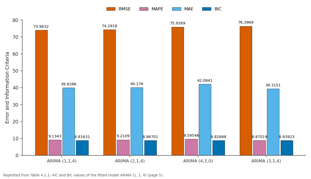
RMSE and MAPE and more: ARIMA (1,1,4) vs ARIMA (2,1,4) vs ARIMA (4,1,0) vs ARIMA (3,1,4)
Replotted from Table 4 (page 5) of the original paper. Every bar is the paper's own table value.
View source evidence ↗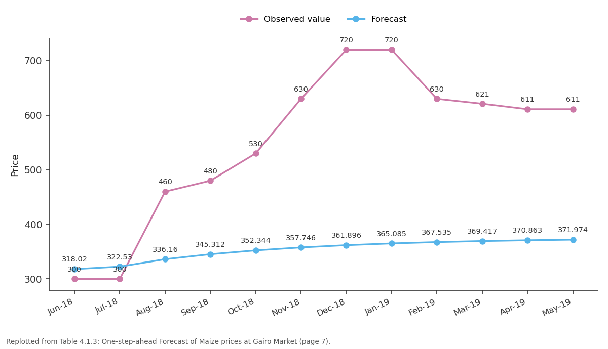
Observed value and Forecast: Jun-18 vs Jul-18 vs Aug-18 vs Sep-18 vs Oct-18
Replotted from Table 4 (page 7) of the original paper. Every bar is the paper's own table value.
View source evidence ↗Figures & tables
From the original paper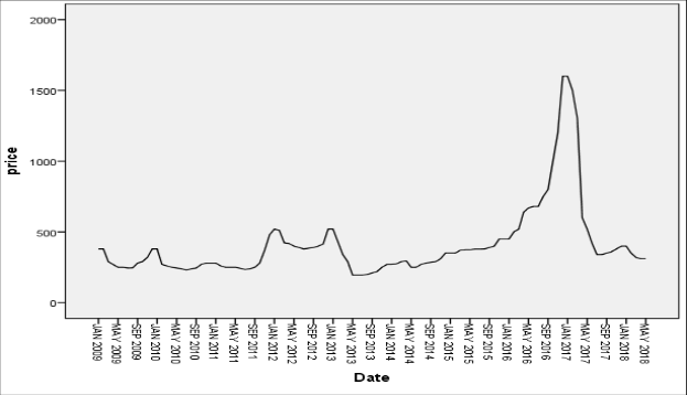 Figure 4Page 3
 Table 4Page 4
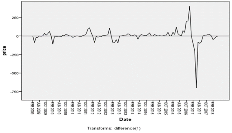 Figure 4Page 4
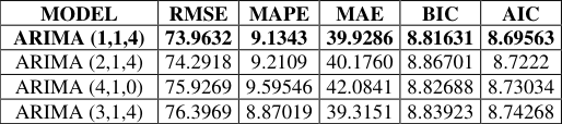 Table 4Page 5
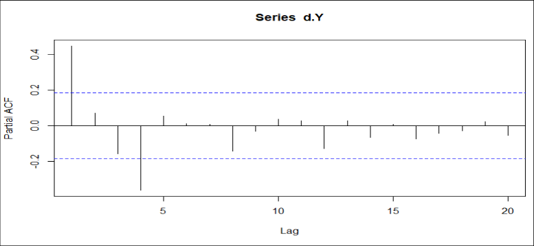 Figure 4Page 5
 Figure 4Page 5
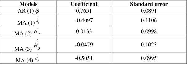 Table 4Page 6
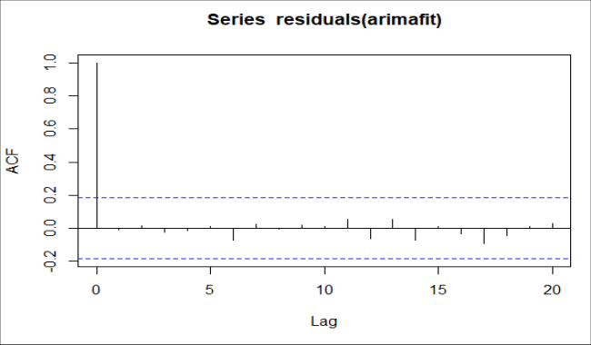 Figure 4Page 6
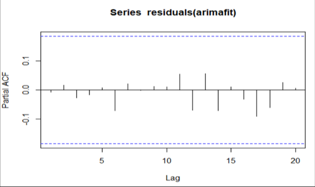 Figure 4Page 6
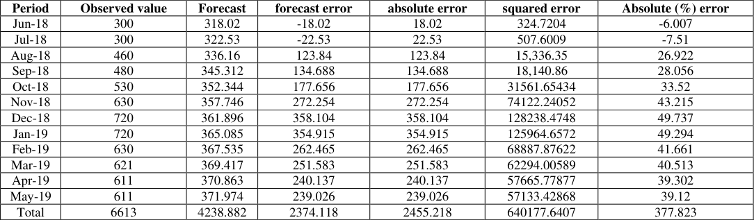 Table 4Page 7
 Table 4Page 7
 Figure 4Page 7
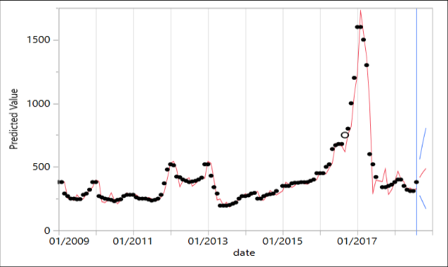 Figure 4Page 8
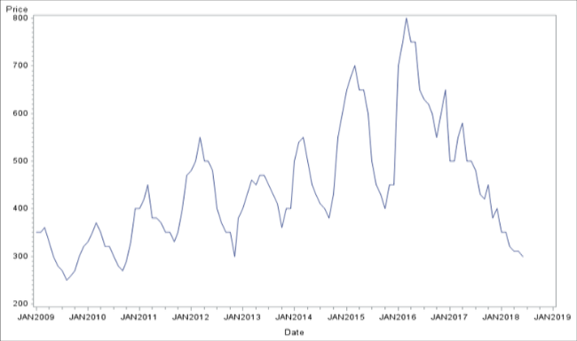 Figure 4Page 8
 Table 4Page 9
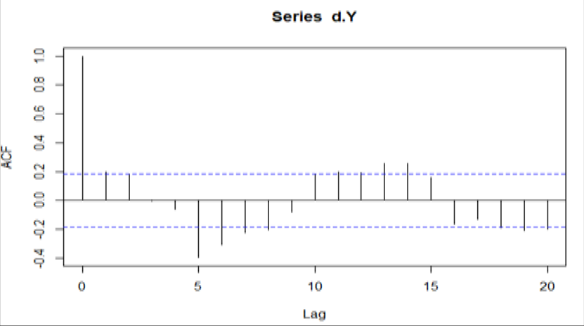 Figure 4Page 9
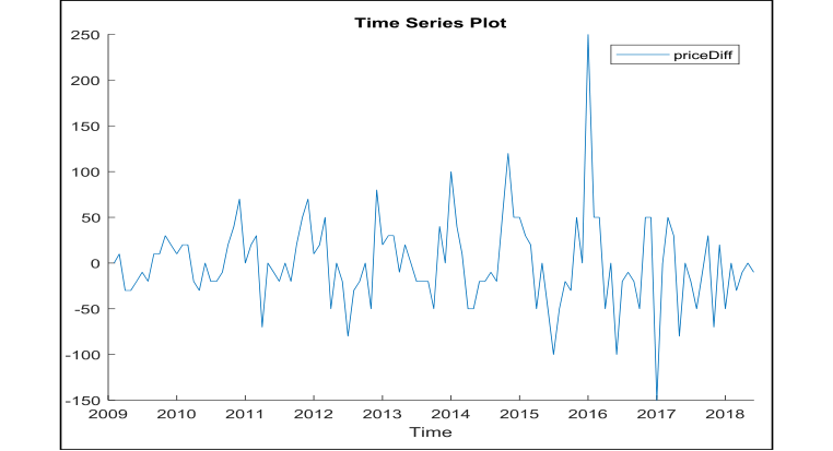 Figure 4Page 9
 Table 4Page 10
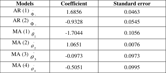 Table 4Page 10
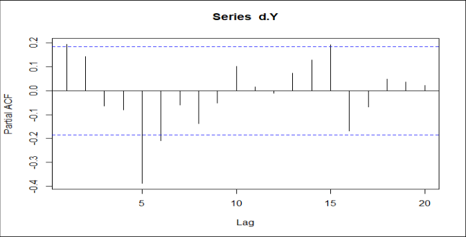 Figure 4Page 10
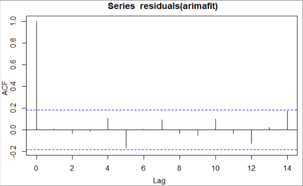 Figure 4Page 11
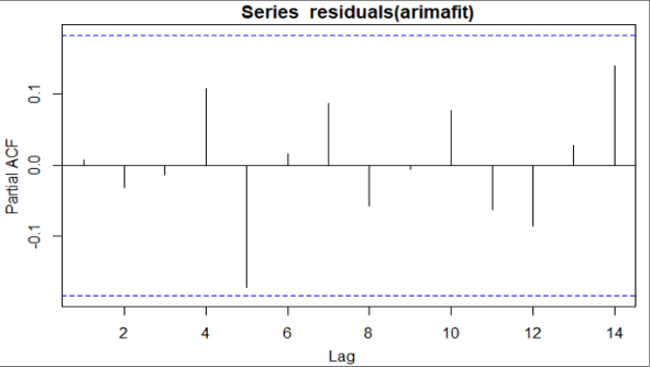 Figure 4Page 11
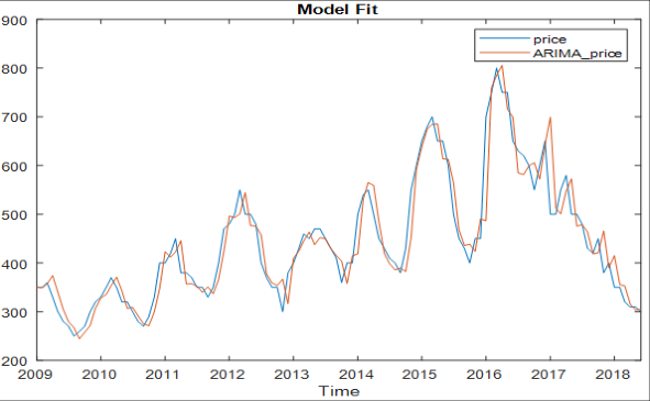 Figure 4Page 11
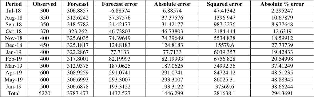 Table 4Page 12
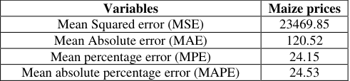 Table 4Page 12
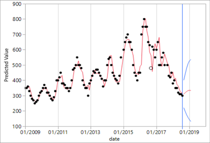 Figure 4Page 12
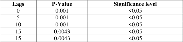 Table 4Page 13
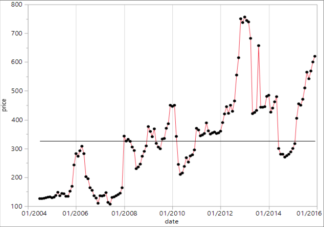 Figure 4Page 13
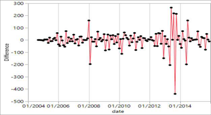 Figure 4Page 13
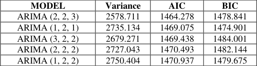 Table 4Page 14
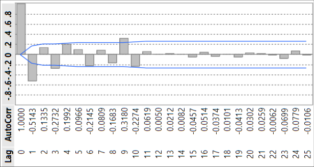 Figure 4Page 14
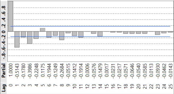 Figure 4Page 14
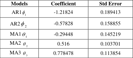 Table 4Page 15
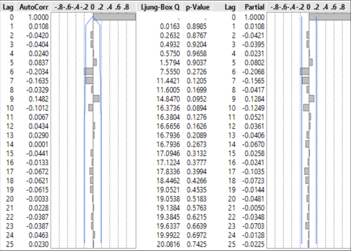 Figure 4Page 15
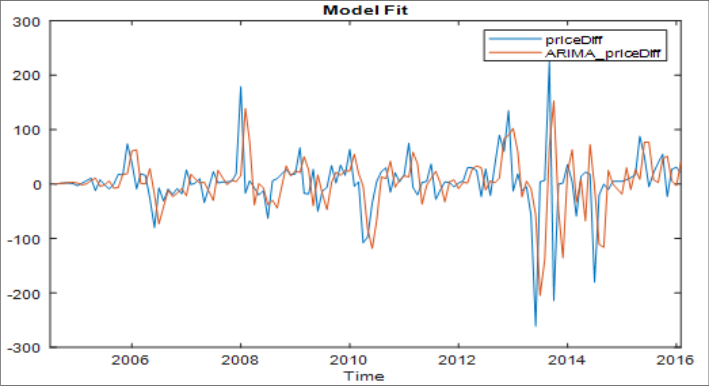 Figure 4Page 15
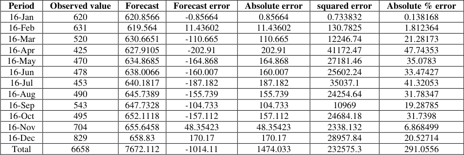 Table 4Page 16
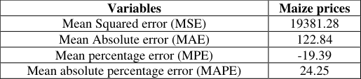 Table 4Page 16
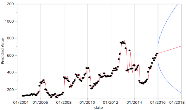 Figure 4Page 16
Introduction
Introduction
Review of Literature Empirical lliterature review outside Tanzania
Several investigators have discussed the use of Univariate time series in modelling and forecasting of various agronomic food crop prices worldwide. The ARIMA technique have been used extensively by a number of researchers to fit model and forecast prices, demands in terms of internal consumption, imports and exports to adopt appropriate solutions. These approaches were employed extensively for forecasting economic time series, inventory and sales modelling also [Ljung and Box (1978) [9] , Pindyck and Rubinfeld (1981) [15] and Sohail et al. (1994)] [18] . Contreras et al. (2003) [4] conducted a study on ARIMA models to predict nextday electricity prices. Rangsan and Nochai (2006) [17] studied oil palm price of Thailand in three categories as farmstead price, general price and wholesome oil palm price by using ARIMA models. Rachana et al. (2010) used ARIMA models to forecast pigeon pea production in India. Badmus and Ariyo (2011) [2] forecasted the area of cultivation and production of maize in Nigeria using ARIMA model. Some more studies on modelling and forecasting by ARIMA were conducted by Adejumo and Momo (2013) [1] , Pierre et al. (2014) [14] , and Gertler et al. (2016) [6] . Kirimi, (2016) [8] conducted study on modelling the volatility of maize prices using ARIMA models so as to achieve the utmost effective and satisfactory model for investigating the unpredictability of prices of maize in Kenya.. Manoj and Anand (2017) [10] studied the application of time series ARIMA forecasting model for predicting sugarcane production in India and found the best ARIMA model as ARIMA (2,1,0). Darekar & Reddy (2017) [5] studied the prediction of paddy prices for Kharif 2017-2018. Venkatesh et al. (2017) [20] studied on the Maize price forecasting by using ARIMA. Nyangarika et al. (2019) [13] has done a study on oil prices factors for forecasting by ARIMA model and forecasts using exponential smoothing.
Time series components analysis
The components of the time series under this study were examined by making time series plots and then seasonal decomposition. Time series plots can detect whether the data are stationary or non-stationary and the plots can help the researcher to recognize the form of essential pattern of the specified data well-arranged over time.
The steps in ARIMA model building A. Plotting of time series data This is done through initial plotting of the historical data and observing its graph whether it is stationary or non-stationary. Plotting the graphs of Autocorrelation Function (ACF) and Partial Autocorrelation Function (PACF) of the historical data helps in identifying if the data existing are stationary or nonstationary.
B. Test for time series stationarity
This test decides whether the series is fixed or not by seeing the ACF graphs. If the ACF graph of past standards either cuts off equally rapidly or passes on down equally rapidly, then the past standards should be used as fixed. If the ACF graph pass on down unhurriedly, then the past values should be used as non-fixed. If the series is not fixed, it can be transformed to a fixed series by differencing. That is, the innovative series is substituted by a series of differences. An ARMA model is formerly stated for the differencing series. Differencing is completed till a plot of the data displays the series fluctuating approximately to a static level, and the graph of ACF is either cut off equally or passes on down equally rapidly. when the special effects of additional time lag 1, 2 , 3, ..., 1 p are eradicated. Partial autocorrelation function (PACF) and autocorrelation function (ACF) can show whether the series is non-stationary by suggesting the type of the model whether it is AR, MA, and ARMA after checking the cutoff of the lag. Model for non-seasonal series are known as Autoregressive Integrated Moving Average model signified by ARIMA (p, d, q). At this point, p specifies the order of autoregressive part, d identifies the amount of differencing and q means the order of the moving average part. If the innovative series is fixed d=0 then ARIMA models diminish to ARMA models. The change linear operator is demarcated by
C. The Augmented
.When the fixed series has been achieved, then classify the formula of the model to be used by means of the graph of autocorrelation function (ACF) and the sample partial autocorrelation function (PACF).
Model Estimation
The procedures are unified by statistical software used for the estimation of the parameters in the model. After reviewing the ACF and PACF, the stationary ARMA, ARIMA and SARIMA can be predicted. In this study, the researcher applied the maximum likelihood technique to estimate the parameters by using the MINTAB and SAS software.
Model checking
Model checking
Bayesian Information Criterion (BIC)
The Bayesian Information Criterion (BIC) projected by Schwarz (1978) is an alternative measure, which tries to precise the AIC's propensity to over-fit. This measure is specified as weakness for the added parameters. As per all measures, the chosen model is the one which has a least BIC.
a) ACF and PACF plots of residuals
As soon as the proper ARIMA model is fitted, the goodness of fit is ascertained by means of plotting the ACF and PACF plots of residuals of the fitted model. If the best sample autocorrelation coefficients of the residuals are inside the limits 1 .9 6 / N where N is the number of observations upon which the model is built, then the residuals are white noise specifying that the model is a good fit.
b) Analysis of autocorrelations of residuals by Box-Pierce or Ljung-Box test
The Ljung -Box test, is useful to the residuals once an ARIMA model has been fixed to check for the uncertainty in the residuals. The Ljung -Box test is built on the autocorrelation plot. However, as a substitute of checking for uncertainty to each distinct lags, it checks the "general" uncertainty based on number of lags.
Forecasting
Forecasting speaks of the estimation of upcoming values of a variable from the historical and present values of that variable or other interrelated variables. This includes the use of the fitted model for estimating the upcoming standards, which can be short-term, medium term and long term predicting. The estimated values are described with confidence intervals listed with the level of significance for out of sample predictions.In prediction, the targeted point is to predict the upcoming values of historical details n m y , where n and m are both constant
based on the data given. Therefore, if the model satisfies all the diagnostic checks, it is well-thought-out for predictions.
Validity
According to Gachengo, (2015) validity helps to increase accuracy, which is useful to the findings by removing as many confounding variables as possible. Finally, analysis was made using Statgraphics, Excel, R software and SAS JPM to ensure both reliability and validity of the outcomes.
Results and Discussion Model Fitting on the Maize Prices for Gairo Market in Morogoro
Model Identification for Gairo Market In modelling, the maize prices time series, the data set of the last twelve months (June 2018 to May 2019) were used for comparing forecast and the modelling was done using the monthly maize prices data from January 2009 to May 2018.
Test for stationary ADF Test
Using ADF test, there is null hypothesis ( ) )
where by o H represents non-stationary time series data while 1 H represents the stationary time series data. The hypothesis is tested by carrying out appropriate differencing of the data in the d th order and applying the ADF test to the differenced time series data. The first order differencing of the data (d=1) means the table of differenced data of current and previous one 1 ( )
is created. The ADF test results are presented in Table 4.1.1. For maize prices at Gairo market, the ADF test statistic in Table 4.1.1 is less than 0.05 p-value for lag order 0 to 15 showing that the series is stationary. Therefore, it is not necessary to add another differencing and ARIMA (p, d, q) is adopted where d=1. This step is essential since it is helpful in further steps for ARIMA (p, 1, q) that is, in finding suitable p in AR and q in MA process. Now, the next step is to examine Autocorrelation Function (ACF) and Partial Autocorrelation Function (PACF). The above ACF infers that the autocorrelation at lag 1 and lag 2 exceed the significance limits and autocorrelation tails off to zero after lag 6. The autocorrelation at lag 3, lag 7 up to lag 20 does not exceed the significant limits. Therefore, it is concluded that those outside the significant limits are assumed as errors that happened by chance. Based on AIC and BIC values, the best model was found to be ARIMA (1, 1, 4). Hence, this is the best model for predicting future values of maize prices at Gairo market. (1 )
| Variables | Maize prices |
|---|---|
| Mean Squared error (MSE) | 19381.28 |
| Mean Absolute error (MAE) | 122.84 |
| Mean percentage error (MPE) | -19.39 |
| Mean absolute percentage error (MAPE) | 24.25 |
Table text extracted from the original PDF; superscript letters are shown inline. The original table image is below.
View original table image
| Period | Observed value | Forecast | Forecast error | Absolute error | squared error | Absolute % error |
|---|---|---|---|---|---|---|
| 16-Jan | 620 | 620.8566 | -0.85664 | 0.85664 | 0.733832 | 0.138168 |
| 16-Feb | 631 | 619.564 | 11.43602 | 11.43602 | 130.7825 | 1.812364 |
| 16-Mar | 520 | 630.6651 | -110.665 | 110.665 | 12246.74 | 21.28173 |
| 16-Apr | 425 | 627.9105 | -202.91 | 202.91 | 41172.47 | 47.74353 |
| 16-May | 470 | 634.8685 | -164.868 | 164.868 | 27181.46 | 35.0783 |
| 16-Jun | 478 | 638.0066 | -160.007 | 160.007 | 25602.24 | 33.47427 |
| 16-Jul | 453 | 640.1817 | -187.182 | 187.182 | 35037.1 | 41.32053 |
| 16-Aug | 490 | 645.7389 | -155.739 | 155.739 | 24254.64 | 31.78347 |
| 16-Sep | 543 | 647.7328 | -104.733 | 104.733 | 10969 | 19.28785 |
| 16-Oct | 495 | 652.1118 | -157.112 | 157.112 | 24684.18 | 31.7398 |
| 16-Nov | 704 | 655.6458 | 48.35423 | 48.35423 | 2338.132 | 6.868499 |
| 16-Dec | 829 | 658.83 | 170.17 | 170.17 | 28957.84 | 20.52714 |
| Total | 6658 | 7672.112 | -1014.11 | 1474.033 | 232575.3 | 291.0556 |
Table text extracted from the original PDF; superscript letters are shown inline. The original table image is below.
View original table image
| MODEL | Variance | AIC | BIC |
|---|---|---|---|
| ARIMA (2, 2, 3) | 2578.711 | 1464.278 | 1478.841 |
| ARIMA (1, 2, 1) | 2735.134 | 1469.075 | 1474.901 |
| ARIMA (3, 2, 2) | 2679.271 | 1469.438 | 1484.001 |
| ARIMA (2, 2, 2) | 2727.043 | 1470.493 | 1482.144 |
| ARIMA (1, 2, 2) | 2750.404 | 1470.937 | 1479.675 |
Table text extracted from the original PDF; superscript letters are shown inline. The original table image is below.
View original table image
| Lags | P-Value | Significance level |
|---|---|---|
| 0 | 0.001 | <0.05 |
| 5 | 0.001 | <0.05 |
| 10 | 0.001 | <0.05 |
| 15 | 0.0043 | <0.05 |
| 15 | 0.0043 | <0.05 |
Table text extracted from the original PDF; superscript letters are shown inline. The original table image is below.
View original table image
| Variables | Maize prices |
|---|---|
| Mean Squared error (MSE) | 23469.85 |
| Mean Absolute error (MAE) | 120.52 |
| Mean percentage error (MPE) | 24.15 |
| Mean absolute percentage error (MAPE) | 24.53 |
Table text extracted from the original PDF; superscript letters are shown inline. The original table image is below.
View original table image
| Period | Observed | Forecast | Forecast error | Absolute error | Squared error | Absolute % error |
|---|---|---|---|---|---|---|
| Jul-18 | 300 | 306.8857 | -6.88574 | 6.88574 | 47.41342 | 2.295247 |
| Aug-18 | 350 | 312.6242 | 37.37576 | 37.37576 | 1396.947 | 10.67879 |
| Sep-18 | 350 | 318.5782 | 31.42177 | 31.42177 | 987.3276 | 8.977648 |
| Oct-18 | 370 | 323.262 | 46.73803 | 46.73803 | 2184.444 | 12.6319 |
| Nov-18 | 400 | 325.6035 | 74.39649 | 74.39649 | 5534.838 | 18.59912 |
| Dec-18 | 450 | 325.1817 | 124.8183 | 124.8183 | 15579.6 | 27.73739 |
| Jan-19 | 400 | 322.2867 | 77.7133 | 77.7133 | 6039.357 | 19.42833 |
| Feb-19 | 400 | 317.8001 | 82.19993 | 82.19993 | 6756.828 | 20.54998 |
| Mar-19 | 500 | 312.9375 | 187.0625 | 187.0625 | 34992.36 | 37.41249 |
| Apr-19 | 600 | 308.9259 | 291.0741 | 291.0741 | 84724.12 | 48.51235 |
| May-19 | 600 | 306.6993 | 293.3007 | 293.3007 | 86025.31 | 48.88345 |
| Jun-19 | 500 | 306.6878 | 193.3122 | 193.3122 | 37369.6 | 38.66244 |
| Total | 5220 | 3787.473 | 1432.527 | 1446.299 | 281638.1 | 294.3691 |
Table text extracted from the original PDF; superscript letters are shown inline. The original table image is below.
View original table image
| Model | AIC | BIC |
|---|---|---|
| ARIMA (2,1,2) Model | 1188.0578 | 1201.6054 |
| ARIMA (2,1,3) Model | 1186.5837 | 1202.8409 |
Table text extracted from the original PDF; superscript letters are shown inline. The original table image is below.
View original table image
| Lags P | -Value | Significance level |
|---|---|---|
| 0 | 0.001 | <0.05 |
| 5 | 0.001 | <0.05 |
| 10 | 0.001 | <0.05 |
Table text extracted from the original PDF; superscript letters are shown inline. The original table image is below.
View original table image
| Variables | Maize Prices |
|---|---|
| Mean Squared error (MSE) | 53348.14 |
| Mean Absolute error (MAE) | 204.60 |
| Mean percentage error (MPE) | 31.49 |
| Mean absolute percentage error (MAPE) | 33.74 |
Table text extracted from the original PDF; superscript letters are shown inline. The original table image is below.
View original table image
| Period | Observed value | Forecast | forecast error | absolute error | squared error | Absolute (%) error |
|---|---|---|---|---|---|---|
| Jun-18 | 300 | 318.02 | -18.02 | 18.02 | 324.7204 | -6.007 |
| Jul-18 | 300 | 322.53 | -22.53 | 22.53 | 507.6009 | -7.51 |
| Aug-18 | 460 | 336.16 | 123.84 | 123.84 | 15,336.35 | 26.922 |
| Sep-18 | 480 | 345.312 | 134.688 | 134.688 | 18,140.86 | 28.056 |
| Oct-18 | 530 | 352.344 | 177.656 | 177.656 | 31561.65434 | 33.52 |
| Nov-18 | 630 | 357.746 | 272.254 | 272.254 | 74122.24052 | 43.215 |
| Dec-18 | 720 | 361.896 | 358.104 | 358.104 | 128238.4748 | 49.737 |
| Jan-19 | 720 | 365.085 | 354.915 | 354.915 | 125964.6572 | 49.294 |
| Feb-19 | 630 | 367.535 | 262.465 | 262.465 | 68887.87622 | 41.661 |
| Mar-19 | 621 | 369.417 | 251.583 | 251.583 | 62294.00589 | 40.513 |
| Apr-19 | 611 | 370.863 | 240.137 | 240.137 | 57665.77877 | 39.302 |
| May-19 | 611 | 371.974 | 239.026 | 239.026 | 57133.42868 | 39.12 |
| Total | 6613 | 4238.882 | 2374.118 | 2455.218 | 640177.6407 | 377.823 |
Table text extracted from the original PDF; superscript letters are shown inline. The original table image is below.
View original table image
| MODEL | RMSE | MAPE | MAE | BIC | AIC |
|---|---|---|---|---|---|
| ARIMA (1,1,4) | 73.9632 | 9.1343 | 39.9286 | 8.81631 | 8.69563 |
| ARIMA (2,1,4) | 74.2918 | 9.2109 | 40.1760 | 8.86701 | 8.7222 |
| ARIMA (4,1,0) | 75.9269 | 9.59546 | 42.0841 | 8.82688 | 8.73034 |
| ARIMA (3,1,4) | 76.3969 | 8.87019 | 39.3151 | 8.83923 | 8.74268 |
Table text extracted from the original PDF; superscript letters are shown inline. The original table image is below.
View original table image
| Lags | P-Value | Significance level |
|---|---|---|
| 0 | 0.001 | <0.05 |
| 5 | 0.001 | <0.05 |
| 10 | 0.0019363 | <0.05 |
| 15 | 0.0011464 | <0.05 |
Table text extracted from the original PDF; superscript letters are shown inline. The original table image is below.
View original table image
Autocorrelation
From this study, the fitted model for maize prices time series data at Gairo market is ARIMA (1, 1, 4). It consists of both AR and MA processes and it is free from seasonal component, which means that seasonality in maize prices is non-significant. The model adequacy is further tested to draw empirical conclusions regarding the model as good fit for forecasting time series. Ljung-box test was done in addition to ACF and PACF residuals plots.
Diagnostic Checking
The diagnostics of the residuals by ACF values in figure 4. 1.5 show that the ACF values are all within the 95% confidence limit indicating that there is no correlation among residuals.
Forecasting Accuracy of the Fitted Model
To assess the model predicting capability, the standard measures of forecast accuracy were obtained as shown in Table 4.1.5. The values of these measures were obtained using the formulae stated in methodological part.
Model Fitting on the Maize Prices for Manyoni Market in SingidaModel Identification for Manyoni Market
In modelling, the maize prices time series, the data set of the last twelve months (June 2018 to May 2019) were used for comparing forecast and the modelling was done using the monthly maize prices data from January 2009 to May 2018. From the plot above, it is concluded that the time series appears to be stationary in both mean and variance. However, before moving to another step, Augmented Dickey-Fuller test was applied to the differenced time series data also for testing stationary.
Test for Stationary ADF Test
Using ADF test, there is null hypothesis For maize prices at Manyoni District, the ADF test statistic in Table 4.2.1 above is less than 0.05 p-value for lag order 0 to 10 showing that the series is stationary, therefore o H is rejected and the conclusion is that the alternative hypothesis is true which means, the series is stationary in both mean and variance. Therefore, it is not necessary to add another differencing and ARIMA (p, d, q) is adopted where d=1. This step is essential since it is helpful in further steps for ARIMA (p, 1, q) in finding suitable p in AR and q in MA process. The above ACF concludes that the autocorrelation at lag 5 exceeds the significance limits and autocorrelation tails off to zero after lag 8. The autocorrelation at lag 13 and lag 14 shows that there is a very low seasonal characteristic that cannot be detected by SPSS. Therefore, it is concluded that those outside the significant limits can be assumed as errors that happened by chance.
Forecasting with the Fitted Model at Manyoni Market
After diagnostic checking, the model fit is used to predict the upcoming values of the variable of interest if it is adequate. But, before forecasting we need to measure the accuracy of its predictions and it is completed by one-step-ahead forecasting.
As a result, the fitted model ARIMA (2, 1, 3) was used to predict the maize prices for twelve months (June 2018-May 2019). The observed and predicted values are shown in Table 4.2.4.
Forecasting Accuracy of the Fitted Model
To assess the model predicting capability, the standard measures of forecast accuracy were obtained as shown in Table 4.2.5. The values of these measures were obtained using the formulae stated in methodological part and the forecast errors existing in Table 4.2.5.
Analysis of Forecasting Errors
The analysis of forecast errors is very important because this aspect is used in evaluating the accuracy of future forecasts of the fitted model. To assess the model forecasting capability, we consider the standard measures of forecast accuracy in H is rejected and the conclusion is that the alternative hypothesis is true which means, the series is stationary in both mean and variance. Therefore, it is not necessary to add another differencing and ARIMA (p, d, q) is adopted where d=1. This step is essential since it is helpful in further steps for ARIMA (p, 1, q) in finding suitable p in AR and q in MA process. Now, the next step is to examine Autocorrelation Function (ACF) and Partial Autocorrelation Function (PACF). The above ACF infers that the autocorrelation at lag 1and lag 3 exceeds the significance limits and autocorrelation tails off to zero thereafter except at lag 9. The autocorrelation, which exceeds the significant limits can be concluded as errors that happened by chance. It is concluded that PACF exceeds significant limits at lag 1 and lag 3, after lag 8 PACF tails off to zero. Those outside the significant limit can be assumed as errors that happened by chance because all PACFs from lag 9 to 25 are within the significant limits. The ACF tailing off to zero after lag 9 and the PACF tailing off to zero after lag 8 can define the following possible ARIMA models for the first differenced time series data of maize prices at Kibaigwa market. where the estimates of parameters are found as 𝜑 ̂1 = -1.2182 𝜑 ̂2 = -0.5783, 𝜃 ̂1 = -0.2945, 𝜃 ̂2 = 0.5160, 𝜃 ̂3 = 0.7785. Hence the estimated equation for ARIMA (2, 2, 3) is obtained as
Autocorrelation
Autocorrelation
References
21 in the original paper- Adejumo AO, Momo AA. Modeling Box-Jenkins Methodology on Retail Prices of Rice in Nigeria, Int. J. Eng. Sci. 2013; 2(9):75-83.
- Badmus MA, Ariyo OS. Forecasting cultivated areas and production of maize in Nigeria using ARIMA model. Asian J Agric. Sci. 2011; 3(3):171-176.
- Box GEP, Jenkin GM. Time Series of Analysis, Forecasting and Control, Sam Franscico, Holden-Day, California. USA, 1976.
- Contreras J, Espínola R, Nogales FJ, Coneja AJ. ARIMA Models to Predict Next-Day Electricity Prices. IEEE Transactions on power systems. 2003; 18(3):1014-1020.
- Darekar A, Reddy AA. Forecasting of Common Paddy Prices in India, J Rice Research. 2017; 10(1):71-75.
- Gertler P, Martinez S, Rawlings LB, Premand P, Vermeersch CMJ. Impact Evaulation in Practice, 2016. Doi.Org/10.1109/WI-IATW.2006.145
- Kibona SE, Mbago MC. Forecasting Wholesale Prices of Maize in Tanzania Using Arima Model, 2017. https://doi.org/10.31559/glm2018.4.3.6
- Kirimi J. Modelling the Volatility of Maize Prices Using Autoregressive Integrated Moving Average Model. Mathematical Theory and Modeling. 2016; 6(6):143-149. www.iiste.org,ISSN 2224-5804 (Paper) ISSN 2225-0522 (Online)
- Ljung GM, Box GEP. On a measure of lack of fit in time series models. Biometrika. 1978; 65:67-72.
- Manoj K, Anand Madhu. An Application of Time Series ARIMA Forecasting Model for Predicting Sugarcane Production in India. Studies in Business and Economics, 2017, 81-94.
- Nkonya E, Xavery P, Akonaay H, Mwangi W, Anandajayasekeram P, Verkuijl H. Adoption of Maize Production Technologies in Northern Tanzania. Mexico D.F: International Maize and Wheat Improvement Center (CIMMYT), The United Republic of Tanzania, and the Southern African Center for Cooperation in Agricultural Research (SACCAR), 1998. ISBN: 970-648-003-X
- Nathaniel Katinila H, Verkuijl W, Mwangi P, Anandajayasekeram, Moshi AJ. Adoption of Maize Production Technologies in Southern Tanzania. Mexico, D.F.: International Maize and Wheat Improvement Center (CIMMYT), the United Republic of Tanzania, and the Southern Africa Centre for Cooperation in Agricultural Research (SACCAR), 1998.
- Nyangarika A, Mikhaylov A, Richter UH. Oil Price Factors : Forecasting on the Base of Modified AutoRegressive Integrated Moving Average Model. International Journal of Energy Economics and Policy. 2019; 9(1):149-159. ISSN: 2146-4553.
- Pierre G, Morales-Opazo C, Demeke M. Analysis and determinants of retail and wholesale staple food price volatility in developing countries, Scientific. January 2014, Food and Agricultural Organization of the UN (FAO), 2014, 3.
- Pindyck RS, Rubinfeld DL. Econometric Models and Economic Forecasts, McGraw-Hill, 1981.
- Rachana W, Suvarna M, Sonal G. Use of ARIMA models for forecasting pigeon pea production in India. Int. Rev. Bus. Financ. 2010; 2(1):97-107.
- Rangsan Nochai, Titida Nochai. ARIMA model for forecasting oil palm price, Proceedings of the 2nd IMTGT Regional Conference on Mathematics, Statistics and Applications, Universiti Sains Malaysia, Penang, 2006.
- Sohail A, Sarwar A, Kamran M. Forecasting total food grains in Pakistan. Department of Math and Stat, University of Agriculture, Faisalabad. J Eng. Appl. Sci. 1994; 13:140-146.
- Urassa Justin K. Factors influencing maize crop production at household levels: A case of Rukwa Region in the southern highlands of Tanzania, African Journal of Agricultural Research. 2015; 10(10):1097-1106.
- Venkatesh Panasa R, Vijaya Kumari, Ramakrishna G, Kaviraju S. Maize Price Forecasting Using Auto Regressive Integrated Moving Average (ARIMA) Model, International Journal of Current Microbiology and Applied Sciences. 2017; 6(8):2887-2895, ISSN: 23197706
- Waryoba FD. Supply Response of Maize in Tanzania Supply Response of Maize in Tanzania MA. (Economics) Dissertation University of Dar Es Salaam, 2015. Https://Doi.Org/10.13140/RG.2.1.1454.4720.