Solving a cash flow oriented EOQ model under permissible delay in payment using Matlab

In this paper an inventory model to determine an optimal ordering policy for non-determining items and time dependent demand rate with delay in payments permitted by the supplies under inflation and time discounting. The permissible delay period ≤ replacement cycle period for setting the account. The objective is minimize the total present value of the cost over time horizon using MATLAB program.

Illustrations explain the paper; they do not show study data.

AI-generated illustration

↗ Enlarge

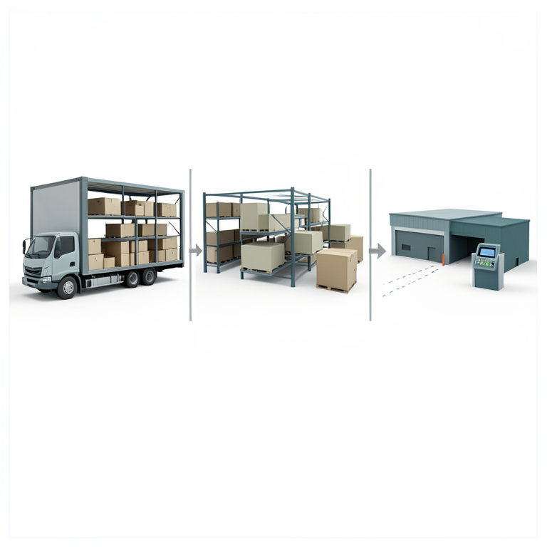
Inventory Model FlowClose ×

AI-generated conceptual illustration (Warehouse inventory of industrial components). It explains the idea and does not show study data.

Open full-size image ↗

Introduction

The Inventory is generally used to indicate raw materials in process, finished product, packaging, spaces and other stocked in order to meet an expected demand or distribute in future. The inventory model with cash flow oriented and quantity dependent under Trade credit is solved analytically to obtain the optimal solution, and Numerical illustration for case m ≤ T is established using MATLAB program 2. Assumptions The following assumptions are used to develop the mathematical model  The demand R (t) for the item is a downward sloping function of the time. For simplicity, we assume that demand is a function of time. i.e.

R (t)=(a+bt) where a>0 and b>0.  Shortages are not allowed.  Lead time is zero.  The net discount rate of inflation rate is constant. 3. Notations The inventory system involves item.  I(t) = Inventory level at time t  Q = Order quantity, units per cycle  H = Length of planning horizon  T = Replenishment cycle time  n = Number of replenishment during the planning horizon, n=H/T  R(t) = Demand rate per unit time, and R(t)=a + bt, a>0, b>0  A0 = Ordering cost at time ‘t’ is zero, $/order  c = Per unit cost of the item, $/unit  h = Inventory holding cost per unit per unit time excluding interest charges, $.unit/unit time  r = Discount rate represent the time value of money  f = Inflation rate  k = The net discount rate of inflation, k = r-f  Ie = The interest earned per dollar in stocks per unit time by the supplies  Ic = The interest charged per dollar in stocks per unit time by the supplies, Ic Ie  m = The permissible delay in settling the account  ip = Interest payable during the first replenishment cycle Maths 2018; 3(2): 607-613 T Jagan Assistant Professor, Department of mathematics, KG college of Arts and science, Coimbatore, Tamil Nadu, India Correspondence T Jagan Assistant Professor, Department of mathematics, KG college of Arts and science, Coimbatore, Tamil Nadu, India  Ip = The total interest payable over the time horizon H  E = Interest earned during the first replenishment cycle  E1 = The present value of the total interest earned over the time horizon H  Z1 (n) = The total present value of the costs over the time horizon H, for m  Z2(n) = The total present value of the costs over the time horizon, form >T= 4. Mathematical Model The inventory I (t) at any time t is depleted by the effect of demand only. Thus the variation of I (t) with respect to‘t’ is governed by the following differential equation. = - (a + bt), 0 T= (1) With the boundary condition I (T) = 0.

The solution of equation (1) is given by I (t) =a (T-t) + (2) The initial inventory (order quantity) after replenishment is given by Q = I (0) = aT + ( (3) The present value of the total replenishment cost is given by (4) The present value of the total purchasing costs is given by (5) The present value of the total holding costs over the time horizon H is given by A = (6) =h =h (7) = = (8) Case I: m The present value of the interest payable during the first replenishment cycle is given by = = = (9) Sub (9) in (8) = = (10) Hence, the present value of the total interest payable over the time horizon H is given by (11) Also, the present value of the interest earned during the first replenishment cycle is E = = = = (12) = = = (13) = b = (14) Sub (12), (13) in (14) E = = (15) Thus the present value of the total interest earned over the time horizon H is =E (16) Therefore, the total present value of the costs over the time horizon H is (17) Differentially equation (17) partially with respect ‘n’ two times, we get (18) Consequently, for fixed ‘H’ is a convex function of ‘n’. Thus there exists a unique value of ‘n’ which minimizes V. Numerical Illustation Case I: M To illustrate this model we consider the following example in which various parameters can be taken as follow A0 = 50 h = 2.0 c = 10 k = 0.10 Ic = 0.15 Ie = 0.12 H = 5 The above illustration is solved by using MATLAB program 1. MATLAB Program clc; closeall; clearall; warningoffall; a=600; b=0.4; A0=50; k=0.1; h=2.0; c=10; Ic=0.15; Ie=0.12; H=5; m=0.1918; n=15:25; for i=1:11 T (i) =H/n (i); Q (i) = ((a*T (i)) + ((b*T (i) ^2)/2)); s0 (i) = ((1-exp (-k*H))/ (1-exp (-k*T (i)))); C1 (i) = A0*s0 (i); C2 (i) = c*Q (i)*s0 (i); A1 (i) = ((exp (-k*T (i))-1)/k); a1 (i) = (T (i)*exp (-k*T (i))); a3 (i) = h/k; a4 (i) = b/k; a2 (i) = a4 (i)*(a1 (i) + A1 (i)); A2 (i) = a3 (i)*(Q (i) + a*A1 (i) +a2 (i)); A (i) =A2 (i)*s0 (i); ip1 (i) = (exp (-k*m)-exp (-k*T (i)))/k; ip2 (i) = ((T (i)*exp (-k*T (i))-(m*exp (-k*m))))/k; ip3 (i) = (exp (-k*T (i))-exp (-k*m))/(k^2); ip4 (i) = (Q (i)*ip1 (i)) + (a*ip2 (i)) + (a*ip3 (i)); ip5 (i) = ((T (i)^2)*exp (-k*T (i))-((m^2)*exp (-k*m)))/k; ip6 (i) = ((T (i)*exp(-k*T (i)))-(m*exp (-k*m)))/(k^2); ip7 (i) = (exp (-k*T (i))-exp (-k*m))/ (k^3); ip8 (i) = (b/2)*(ip5(i)+(2*ip6(i))+(2*ip7(i))); ip (i) = (c*Ic* (ip4 (i) + ip8 (i))); Ip (i) = ip (i)*s0 (i); E1 (i) = ((-T (i)*exp (-k*T (i)))/k) + (1-exp (-k*T (i)))/ (k^2); E2 (i) = (((T(i)^2)*exp(-k*T(i)))/k)+((2*T(i)*exp(-k*T(i)))/(k^2))+(2*(exp(-k*T(i))-1)/(k^3)); E (i) = c*Ie*((a*E1 (i))-(b*E2 (i))); E1 (i) = E (i)*s0 (i); z1 (i) = C1 (i) + C2 (i) + A (i) + Ip (i)-E_1 (i); E2 (i) = c*Ie*(((a*E1 (i))-(b*E2 (i)) + (m-T (i))*Q (i)*exp (-k*T (i)))); E3 (i) = E2 (i)*s0 (i); if (m<=T (i)) Z (i) = z1 (i); End End Figure; Plot (Z) Title ('TOTAL COSTS Z (n)') Figure; Plot (T); title ('Replenishment cycle time (T)'); Figure; Plot (Q); Title ('Order quantity (Q)'); 5.

Sensitive Analysis The sensitive analysis shows individual optimal solution different from each other for different values of net discount rate of inflation k and number of replenishment during ‘n’. The minimum total present value of the cost is obtain and when the number of replenishment n=20. The optimal (minimal) order quantity Q=150.01 and the optimal (minimal) total present value of the cost Z=2.4967 Using MATLAB program graphical representation for various parameter. (i) Plot of’’ n’ against total (z (n)) (ii) Plot of’ n’ against T (cycle time) (iii) Plot of ‘n’ against Q VII.

Conclusion

A mathematical model for cash flow oriented EOQ under the permissible delay in payments is solved by numerical example and established using MATLAB program, it works as an effective tool to obtain the optimal number 0f replenishment cycle time and order quantity to replenishment cycle time and order quantity to minimize the total present value of costs. It attracts new customer and also reduce the buys cost of holding cost.

1. Goyal SK. Economic order quantity under conditions of permissible delay in payments, journal of the operational research society. 1985; 36:335-338
2. Ouyang LY, Wu sarker BR, Yang CT. A study on an inventory model for non-instantaneous deteriorating items with permissible delay in payments. comput. ind. Eng. 2006; 637-651.
3. Premkumar Gupta, Hira DS. Operational research, S. chand and Company LTD, 1st edition, 1979.
4. Aggarwal SP, jaggi CK. Ordering polices of deteriorating items under permissible delay in payments, journal of operational research society. 1995; 46:458-462.
5. Jagan T, EOQ for deteriorating item with non- instantaneous receipt under trade credits with shortages, International Journal of Scientific Development and Research. 2(5):2455-2631.