
Research article · 2019 · Full text
International Journal of Statistics and Applied MathematicsForecasting foreign tourist arrivals to India using alternative forecasting combinations
Volume 4(5) · Pages 20–24
Research areasGrey System Theory ApplicationsDiverse Aspects of Tourism ResearchEnergy, Environment, Economic Growth
Abstract
Author-writtenIn this study, Naive I & Naive II, Grey and vector error correction (VEC) models are applied to forecast foreign tourist arrivals (FTAs) to India. Bates and Granger (1969) developed combination of forecasts by using the various combination methods in order to improve the single forecasts accuracy. Therefore, the combination methods based on simple average (SA) and inverse of mean absolute percentage error (IMAPE) is applied to improve the efficiency of individual forecasting methods. The data of FTAs to India from January 2003 to December 2016 obtained from http://www.indiastat.com are used for the overall empirical analysis. The results of the empirical study show that the combination forecasts have a better accuracy than the individual forecasts under root mean square error (RMSE), mean absolute percentage error (MAPE) and U-statistic (U) criteria. The study also demonstrates that the inverse of MAPE combination method is more suitable for forecasting of FTAs than simple average and others time series models.
Summary
Source-checkedPlain-language reading of the full paper, prepared with AI and checked against the text. Each point links to the authors' own words.
Why it matters
- Forecasting air travel demand is valuable for various organizations to help with resource allocation and future planning within the tourism and travel industry. View evidence ↗
- Combining forecast values from multiple time series models is generally believed to yield better performance than relying on a single model. View evidence ↗
The question
- The study aims to forecast foreign tourist arrivals (FTAs) to India using individual time series models and two combination methods: simple average (SA) and inverse of mean absolute percentage error (IMAPE). View evidence ↗
- The research seeks to compare the performance of these individual and combination models using RMSE, MAPE, and U-statistic criteria. View evidence ↗
What they did
- The analysis used monthly data of foreign tourist arrivals to India from January 2003 to December 2016. View evidence ↗
- The data was split into an estimation period (January 2003 to December 2012, 120 observations) and an out-of-sample forecasting period (January 2013 to December 2016). View evidence ↗
- The individual forecasting models applied were Naive I, Naive II, Grey, and Vector Error Correction (VEC). View evidence ↗
- The VEC model incorporated exchange rate (EXR), foreign exchange earnings (FEEs), and tourist arrivals from the USA (USAFTAs). View evidence ↗
What they found
- Among the single time series models, Naive I and VEC demonstrated higher accuracy than Naive II and Grey models. View evidence ↗
- Both the simple average (SA) and inverse of MAPE (IMAPE) combination methods outperformed all individual models across RMSE, MAPE, and U-statistic metrics. View evidence ↗
- The IMAPE combination method was found to be superior to the SA method and all individual time series models. View evidence ↗
- The IMAPE method achieved the lowest error rates, with an RMSE of 27074.2 and MAPE of 3.2%, compared to the worst individual model (Naive II) which had an RMSE of 51498.7 and MAPE of 6.27%. View evidence ↗
What it means
- The authors conclude that combining single forecast values from various time series models improves the overall efficiency of the forecasting process. View evidence ↗
- The authors suggest that forecasting efficiency can be further enhanced by determining the most appropriate weights for the individual models. View evidence ↗
Visual summary
1 visualsIllustrations explain the paper; they do not show study data.

Forecasting Workflow
AI-generated conceptual illustration (A map of India and a digital data stream). It explains the idea and does not show study data.
View source evidence ↗Figures & tables
From the original paper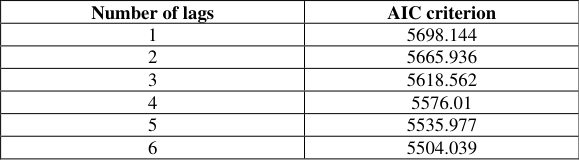 Table 1
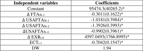 Table 2
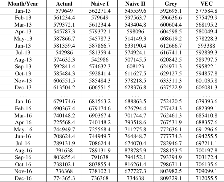 Table 3
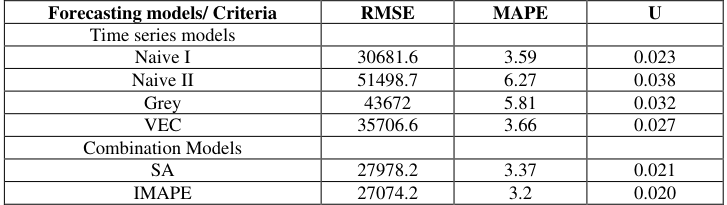 Table 4
Introduction
Modeling and forecasting air travel demand can provide reliable and valuable information for public, private and voluntary sector organizations in allocating resources and for future planning of tourism and the travel industry. Therefore, various univariate time series approaches have been employed in tourism demand modeling and forecasting. For example, Chu (1998) [6] employed various univariate time series models such as Box-Jenkins (Box and Jenkins (1976)) [3] and Holt-Winters for tourism demand forecasting in Asian-Pacific countries. Chen et al. (2009) [8] compared the accuracy of SARIMA model with Holt-Winters and Grey model to forecast inbound air travel arrivals for Taiwan. The other study used multivariate vector error correction models for the forecasting of inbound tourism demand (Kim and Song (1998)) [12] . It is believed that the combination of forecast values obtained from different time series models provides better forecasting performance than that of single forecast value. In this regard, Bates and Granger (1969) [4] developed combination of forecasts by using the various combination methods in order to improve the single forecasts accuracy. Combination of forecasts is a combination of single forecasts produced from various models which provides more precise and accurate forecast value than that of individual models, depending on the combination techniques (Clemen, 1989, Trabelsi and Hillmer, 1989, Makridakis and Hibon, 2000, Stock and Watson, 2004, Aiolfi and Timmermann, 2006) [5,16,1] . Further, selection of suitable weight coefficient is the greatest concern in forming the combination of forecast (or forecast combination). A vast literature has employed various methods to obtain the accurate weight coefficient in forming the combination of forecasts. For example, Russell and Adam (1987) [17] and Schwaerzel and Rosen (1997) evaluated the weight coefficient by utilizing mean square error, mean absolute error and mean absolute percentage error. Similarly, Menezes et al. (2000) [15] presented a detailed review on combination approaches and used the simple average, regression-based methods and the switching method. Also, Chan et al. (2004) [7] applied quality control methods for the evaluation of weights to forecast product demand. Rong (2007) [18] applied a combination methods based on inverse of exponentially weighted moving average (EWMA) and mean absolute percentage error (MAPE) of each individual forecasting models.
The results of an empirical analysis shows that the combination methods have a better accuracy than the generalized autoregressive conditional heteroscedasticity (GARCH), exponential generalized autoregressive conditional heteroscedastic (EGARCH) and random walk models. Recently, Song et al. (2011) used induced order weighted averaging operator (IOWA) method to combine forecasting results of Grey and other time series models for forecasting of energy consumption of Hebei Province. The empirical evidence shows that performance of combination method is better than individual methods when compared under suitable selection criterion. It has been observed that the combination of forecasts has not been much studied in the tourism demand forecasting in recent years. A few number of studies applied combination of forecast in tourism demand forecasting. For example, Shen and Li (2008) evaluated the forecasting performance of different combination methods to forecast tourism demand for the USA. Andrawis et al. (2011) [2] explains a detail review on various combination techniques for short-term and long-term tourism demand forecasting. The empirical results also confirm the better performance of the proposed combination approach. Also, Lu et al. (2015) [14] applied the concept of induced order weighted averaging operator (IOWA) to combine the forecasting results of ARIMA and Grey model in tourism demand forecasting. It is found that the combination approach has better forecasting performance than that of individual models. In this paper, forecasting of FTAs to India has been done by using time series forecasting models and the combination methods: simple average (SA) and inverse of mean absolute percentage error (IMAPE). We compare the forecasting performance of individual and combination models by using root mean square error (RMSE), mean absolute percentage error (MAPE) and U-statistic criteria. The rest of the paper is as follows. Section 2 briefly explains time series and combination models. Section 3 describes the data. Section 4 defines comparison criteria for evaluating the forecasting performance. Section 5 presents the empirical findings and comparison of combination and single methods and the last section gives the conclusions.
Forecasting models
In this section, we discuss the theoretical aspects of individual and combination methods related to FTAs forecasting. The methods are: (i) Naive (ii) Grey (iii) VEC (iv) Combination.
Time series models 2.1.1 Naive model
Naive methods are simple models to forecast time series data. The first method is Naive I and second method is Naive II. Forecasts can be generated by utilizing the previous value of time series data in Naive I method. While in Naive II method forecast of current observation is put equal to the previous value and multiplied by the growth rate of current observation over the previous observation.
Grey model
In time series forecasting, the statistical models require some statistical assumptions. Although, there exist some forecasting models for analyzing the time series data which are free from any statistical limitations such as Grey model developed by Deng (1982) [9] . In time series forecasting accumulated generation operation (AGO) is used to decrease the randomness of the data while applying Grey model. In this model, time series data can be forecasted by using linear differential equation of order one. Also, the parameters of the model can be evaluated through the ordinary least squares (OLS) estimation method. The Grey model of first order linear differential equation is written as
Where, X t is a time series and a & b are the parameters.
Vector error correction model (VEC)
There exist several methods to analyze the relationship between foreign tourist arrivals and their determining factors. If the variable of interest let X t , is related to one or more than one time series variables, then it is possible to develop a model which utilizes information contained in these time series to help forecast X t . It also improves prediction accuracy of X t. . These models are called multivariate time series models. VEC is one of the most commonly applied multivariate econometric model to forecast time series data by utilizing more than one co-integrating relationships for a set of time series variables developed by Engle and Granger (1987) [10] . It is an extension of the univariate time series model to dynamic multivariate time series. The first step in constructing a VEC model is fitting a vector autoregression (VAR) model for a set of K time series variables X t = (X 1t , X 2t ,. . ., X Kt ) . The VAR model of order p is given by
Where, E i (i = 1, 2, . ., p) are (K × K) coefficient matrices and u t = (u 1t , u 2t . . . u Kt ) is assumed to be a vector of independent error. Now, the VEC model is obtained from the VAR by subtracting X t-1 from both sides and rear-ranging the terms.
The form of VEC model can be written as
where, Π = -(I k -A 1 -... -A p ), Γ i = -(A i+1+...+A p ) for i=1,...,p-1 and u t is the error term. Also, the parameters involved in the model can be estimated using the ordinary least squares (OLS) method.
Combination methods
In combination method, the forecasts values are combined by using suitable weight coefficients pro-vided to single forecast value obtained from two or more time series models. The combination of forecast, Yˆc, t is calculated by applying the formula as follows:
Where X m,t ̂ represents the forecast value obtained from the m th time series model. Here, the weights w i are decided on the basis of two methods, simple average (SA) and inverse of MAPE. A brief explanation of these methods is given below.
Simple average (SA)
Simple average method is based on the calculation of average of forecasting values obtained from different time series models. In this method, the weight wi for two or more forecasting models are same, w i =
. Suppose that X 1t , X 2t … X mt are m forecasts values of forecasting models, then the expression for simple average combination method is given by
Inverse of MAPE (IMAPE)
In simple average method, we assume that all the forecasting models in the combination have equal importance. If some models are more important than others in the combination then it is better to apply inverse of MAPE method for the weight calculation. Inverse of MAPE is a combination method in which the weights are calculated based on forecasting performance of time series models. In this method, the weight w i are determined as follows:
Where MAPE j (j = 1, 2, 3...m) is a MAPE obtained for j th time series model. The calculation of MAPE is discussed in Section 4
Data
This study employed the monthly time series data of FTAs (in numbers) from January 2003 to December 2016 in India. Also, the factors like exchange rate (EXR), foreign exchange earnings (FEEs) and tourists arrivals from USA (USAFTAs) are used for the building of VEC model. The data were obtained from the official website of http://www.indiastat.com. The series is transformed by using ratio to moving average method in order to remove the seasonality from the FTAs time series data. The whole time series is divided into two periods (1) 2003:1-2012:12, of 120 observations, to estimate the individual models; (2) data of 2013:1-2016:12 are used to generate the out-of-sample forecasts for different models. The R-3.0.3 software is used for the overall empirical analysis.
Comparison criteria
The forecasting performance of individual and combination models for FTAs time series data has been evaluated using root mean square error, mean absolute percentage error and U-statistic criteria, which are given below:
Root Mean Square Error (RMSE) RMSE is given by
It is a known fact that lowers the value of RMSE better the model is.
Mean absolute percentage error (MAPE)
MAPE is a relative measure of errors in prediction. It usually expresses accuracy as a percentage, and is defined by the following formula
Where n is sample size, X t is actual value of the time series and is the forecast in the t th month.
Note that Lewis (1982) [13] demonstrates that the value of MAPE being less than 10% indicates the high accuracy of forecasting. Moreover, when it lies between 10-20% forecasting is good, 20-50% is reasonable and more than 50% denotes inaccuracy in forecasting.
U-statistic
U statistic is calculated by using the following formula
The value of U lies in the range 0 to 1. U = 0 indicates that the forecasting is highly reliable, and, if U is close to 1, it shows the inaccuracy of forecasting methods.
Empirical findings 5.1 Time series models
In this section empirical results of Naive, Grey and VEC models are evaluated. The estimated values of the parameters a & b for Grey model are -0.006628205 and 266972.1, respectively. Moreover, the order of VEC model has been selected on the basis of minimum AIC value. The results of AIC values for six lags are reported in Table 1. Also, the estimated results of VEC model are reported in Table 2 with the values of t statistics in parenthesis. It can be noticed that coefficient of error correction term (ECT) is found to be significant and negative in the equation at 5% level of significance indicating long run equilibrium relationship among variables. The lags of FTAs, EXR, FEEs and USAFTAs are included in VEC model. However, only significant terms are retained in the estimated equation with the non-significant terms being deleted first. Now the forecasting performance from Naive I & Naive II, Grey and VEC models is evaluated and reported in Table 3. It can be noticed that the forecast values obtained from VEC models are closer to the actual forecast value in all the years than that of other models. Interestingly, when these models are compared under the three criteria, the results obtained are reported in Table 4, VEC model performs better than Naive II and Grey models.
| Forecasting models/ Criteria | RMSE | MAPE | U |
|---|---|---|---|
| Time series models | |||
| Naive I | 30681.6 | 3.59 | 0.023 |
| Naive II | 51498.7 | 6.27 | 0.038 |
| Grey | 43672 | 5.81 | 0.032 |
| VEC | 35706.6 | 3.66 | 0.027 |
| Combination Models | |||
| SA | 27978.2 | 3.37 | 0.021 |
| IMAPE | 27074.2 | 3.2 | 0.020 |
Table text extracted from the original PDF; superscript letters are shown inline. The original table image is below.
View original table image
| Month/Year | Actual | Naive I | Naive II | Grey | VEC |
|---|---|---|---|---|---|
| Jan-13 | 579649 | 562271.4 | 545559.6 | 592695.1 | 577584.8 |
| Feb-13 | 561234.4 | 579649 | 597563.7 | 596636.6 | 575479.9 |
| Mar-13 | 579372.1 | 561234.4 | 543404.8 | 600604.4 | 568195.2 |
| Apr-13 | 545787.3 | 579372.1 | 598096 | 604598.5 | 580049.4 |
| May-13 | 587866.7 | 545787.3 | 514149.3 | 608619.2 | 578228.3 |
| Jun-13 | 581359.4 | 587866.7 | 633190.4 | 612666.7 | 593388 |
| Jul-13 | 542986 | 581359.4 | 574924.1 | 616741.1 | 592839.3 |
| Aug-13 | 574632.3 | 542986 | 507145.5 | 620842.5 | 589797.5 |
| Sep-13 | 592841.4 | 574632.3 | 608123 | 624971.3 | 595822.1 |
| Oct-13 | 585484.3 | 592841.4 | 611627.5 | 629127.5 | 594857.8 |
| Nov-13 | 606551.5 | 585484.3 | 578218.5 | 633311.3 | 601035.8 |
| Dec-13 | 613504.2 | 606551.5 | 628376.8 | 637522.9 | 606081.3 |
| . . . | . . . | . . . | . . . | . . . | . . . |
| Jan-16 | 679174.6 | 681563.2 | 688863.5 | 752420.5 | 679393.6 |
| Feb-16 | 690367.4 | 679174.6 | 676794.4 | 757424.3 | 682399.1 |
| Mar-16 | 740148.2 | 690367.4 | 701744.7 | 762461.3 | 685410.8 |
| Apr-16 | 725568.4 | 740148.2 | 793518.6 | 767531.9 | 688357.6 |
| May-16 | 744949.7 | 725568.4 | 711275.8 | 772636.1 | 691296.6 |
| Jun-16 | 708624.4 | 744949.7 | 764848.7 | 777774.3 | 694255.5 |
| Jul-16 | 789131.9 | 708624.4 | 674070.4 | 782946.7 | 697211.1 |
| Aug-16 | 791638 | 789131.9 | 878785.9 | 788153.5 | 700197.8 |
| Sep-16 | 803855.4 | 791638 | 794152.1 | 793394.9 | 703172.4 |
| Oct-16 | 738102.1 | 803855.4 | 816261.4 | 798671.1 | 706135.6 |
| Nov-16 | 736368 | 738102.1 | 677727.3 | 803982.5 | 709099.1 |
| Dec-16 | 774365.3 | 736368 | 734638 | 809329.1 | 712055.5 |
Table text extracted from the original PDF; superscript letters are shown inline. The original table image is below.
View original table image
| Independent variables | Coefficients |
|---|---|
| Constant | 95474.3(40265.2)* |
| ∆ FTAst-1 | -0.3011(0.1622)* |
| ∆ USAFTAst-1 | -1.0181(0.3984)* |
| ∆ USAFTAst-2 | -1.3926(0.3993)* |
| ∆USAFTAst-4 | -0.9902(0.3961)* |
| ∆ EXRt-6 | 4597.0493(1766.8995)* |
| ECTt-1 | -0.7042(0.1547)* |
| DW | 1.94 |
Table text extracted from the original PDF; superscript letters are shown inline. The original table image is below.
View original table image
| Number of lags | AIC criterion |
|---|---|
| 1 | 5698.144 |
| 2 | 5665.936 |
| 3 | 5618.562 |
| 4 | 5576.01 |
| 5 | 5535.977 |
| 6 | 5504.039 |
Table text extracted from the original PDF; superscript letters are shown inline. The original table image is below.
View original table image
Combination methods
Here, the forecast values of Naive I & Naive II, Grey and VEC models are combined by using the weight coefficients (w i , i = 1,2,3,4) obtained from simple average and inverse of MAPE combination methods. In simple average method, each single forecasts have equal weight while in inverse of MAPE method weights are just inverse of MAPE values. According to the forecasting results of each single model, weights are computed by simple average and inverse of MAPE by using equations ( 4) and (5). Finally, the combined forecasting model using simple average and inverse of MAPE methods is obtained as: X^t = 0.5Naive I + 0.5Naive II + 0.5Grey + 0.5VEC
X^t = 0.278Naive I + 0.159Naive II + 0.172Grey + 0.273VEC (7) Further, the above two combination equations ( 6) and ( 7) are used to forecast FTAs. The forecasting performance of SA and IMAPE combination methods is evaluated by calculating the RMSE, MAPE and U-statistic using the out-of-sample forecasts from January 2013 to December 2016. The results of three criteria are reported in Table 4 for each of the combination methods. As shown in Table 4, the SA and IMAPE combination methods outperform the individual methods due to its lesser RMSE, MAPE and U values. Moreover, the IMAPE combination method is better than the SA and other individual time series models.
References
18 in the original paper- Aiolfi M, Timmermann A. Persistence in forecasting performance and conditional combi-nation strategies, Journal of Econometrics. 2006; 135:3153.
- Andrawis RR, Atiya AF, Shishiny HE. Combination of long term and short term forecasts, with application to tourism demand forecasting, International Journal of Forecasting. 2011; 27:870886.
- Box GEP, Jenkins GM. Time series analysis, Forecasting and Control, 1976.
- Bates JM, Granger CW. The combination of forecasts, Operational Research Quarterly. 1969; 20:451-468.
- Clemen RT. Combining forecasts: a review and annotated bibliography, International Journal of Forecasting. 1989; 5:559583.
- Chu FL. Forecasting tourism demand in Asian-Pacific countries, Annual of Tourism Research. 1998; 25(3):597615.
- Chan CK, Kingsman BG, Wong H. Determinging when to update the weights in combined forecasts for product demand-an application of the C-USUM technique, European Journal of Operational Research. 2004; 153:757-768.
- Chen CF, Chang YH, Chang YW. Seasonal ARIMA forecasting of inbound air travel arrivals to Taiwan, Transportmetrica. 2009; 5(2):125-140.
- Deng J. Control problems of Grey systems, Systems and Control Letters. 1982; 1(1):288-294.
- Engle RF, Granger CWJ. Co-Integration and error correction: representation, estimation, and testing, Econometrica. 1987; 55(2):251-276.
- Greene MN, Howrey EP, Hymans SW. The use of outside information in econometric forecasting, In E. Kuh, and D. A. Belsley (Eds.), Model reliability. Cambridge, MA: MIT Press, 1986.
- Kim S, Song H. Analysis of tourism demand in South Korea: a cointegration and error correction approach, Tourism Analysis. 1998; 3(1):25-41.
- Lewis CD. International and business forecasting methods, London: Butterworths, 1982.
- Lu F, Zhu X, Peng Z, Zhou X. Combination forecast on tourism demands based on IOWA operator, Energy Procedia. 2015; 5:2224-2229.
- Menezes LMD, Bunn DW, Taylor JW. Review of guidelines for the use of combined forecasts, European Journal of Operational Research. 2000; 120:190-204.
- Makridakis S, Hibon M. The M3-competition: results, conclusions, and implications, International Journal of Forecasting. 2000; 16:451-476.
- Russll TD, Adam EE. An empirical evaluation of alternative forecasting combinations, Management Science. 1987; 33(10):1267-1376.
- Rong DJ. Combining stock market volatility forecasts using an EWMA technique, IEEE, 2007, 5272-5275.