
Research article · 2017 · Full text
International Journal of Statistics and Applied MathematicsStochastic models for reservoir inflow simulation
Volume 2(6) · Pages 197–203
Research areasWater resources management and optimizationHydrology and Drought Analysis
Abstract
Author-writtenForecasting of inflow to a new reservoir and modelling of the historical behaviour of an existing reservoir can be accomplished through simulation models. First order stationary Markov model assuming stationary mean, standard deviation and lag1 correlation for the historical and generated data would result in a perfect simulation for annual stream flows and reservoir inflows. Seasonal models can be introduced in which the seasons can be either months, or any intra year period variation and here the inherent periodicity would introduce non stationarity in the data. First order Markov model addressing the non stationarity is a better alternative recommended in this situation. Simulations for Karappara (100 27’ 25”N 760 38’ 51” E) Stream flow and Idamalayar (100 13’ 18” N 760 42’ 21” E) Reservoir Inflow belonging to Kerala state have been realised with respect to both stationary and non-stationary data.
Summary
Source-checkedPlain-language reading of the full paper, prepared with AI and checked against the text. Each point links to the authors' own words.
Why it matters
- Climate change is expected to accelerate the hydrological cycle, which may alter the timing and intensity of rainfall. View evidence ↗
- Reservoirs are used to store surplus rainy season water for irrigation during droughts and to help prevent floods. View evidence ↗
- Simulation models are necessary to obtain precise estimates of reservoir yield. View evidence ↗
The question
- The study aimed to develop stochastic models to simulate stream flow and reservoir inflow using long-term data to reliably anticipate future flows. View evidence ↗
What they did
- A first-order Markov process was employed to model the data, as hydrological flows often show persistence based on the immediate past. View evidence ↗
- To handle non-stationary data, such as monthly flows, the model incorporated variations in mean, standard deviation, and lag1 correlation by year and month. View evidence ↗
What they found
- The historical annual flow at the Karappara weir had a mean of 79.42 Mm3, a standard deviation of 26.81 Mm3, and a lag1 correlation of 0.26. View evidence ↗
- The stationary Markov model generated annual Karappara flows with a mean of 80.37 Mm3, S.D of 25.20 Mm3, and lag1 correlation of 0.35, which were close to historical values. View evidence ↗
- Monthly inflow to the Idamalayar Reservoir was found to be non-stationary and non-normal, requiring logarithmic transformation before fitting the non-stationary Markov model. View evidence ↗
- The non-stationary Markov model for Idamalayar Reservoir produced simulated series that compared well with historical data regarding mean, S.D, and lag1 correlation. View evidence ↗
What it means
- The authors conclude that first-order stationary Markov models are effective for annual flows, while models addressing non-stationarity should be used for monthly inflow data. View evidence ↗
- The models are designed to preserve historical mean, S.D, and lag1 correlation, but they may not accurately reproduce peak flows. View evidence ↗
Visual summary
2 visualsIllustrations explain the paper; charts are replotted from the paper's own table values.
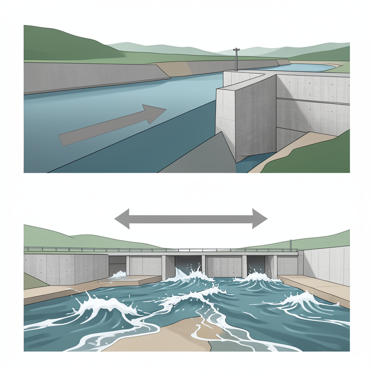
Markov Model Comparison
AI-generated conceptual illustration (A river flowing into a concrete reservoir dam). It explains the idea and does not show study data.
View source evidence ↗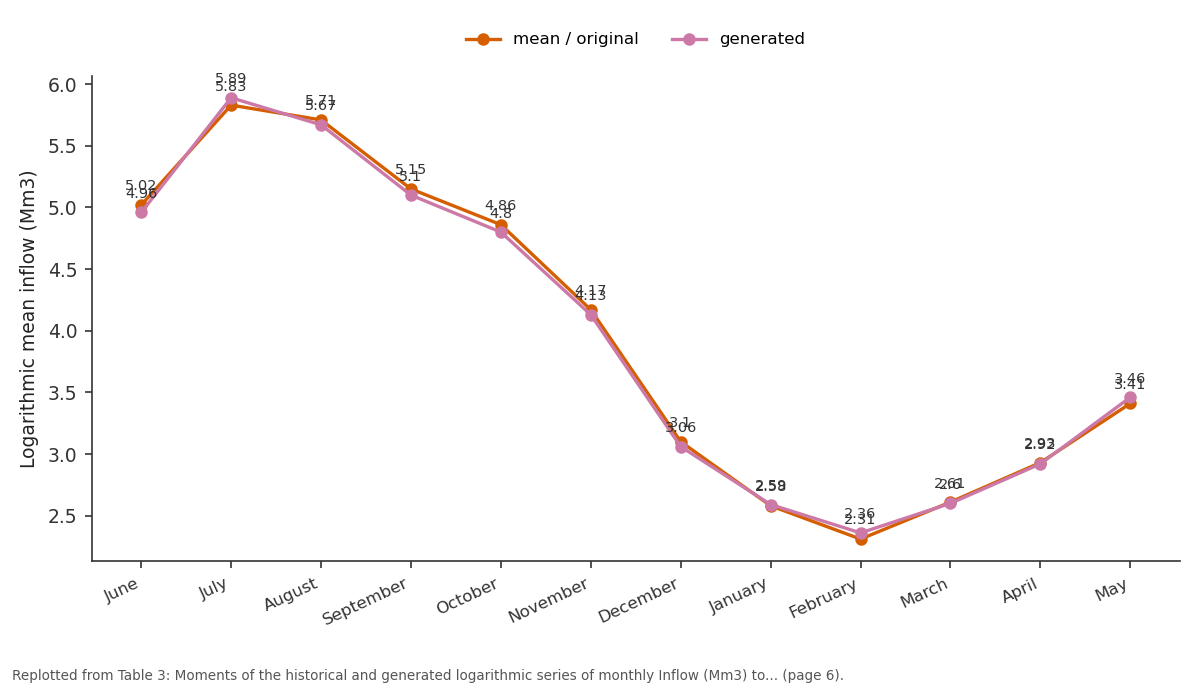
mean / original and generated: June vs July vs August vs September vs October
Replotted from Table 3 (page 6) of the original paper. Every bar is the paper's own table value.
View source evidence ↗Figures & tables
From the original paper Table 1
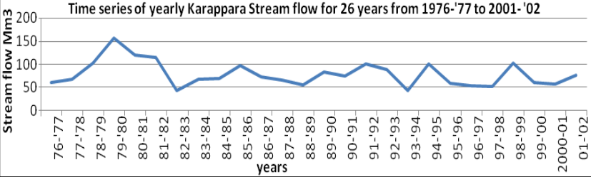 Figure 1
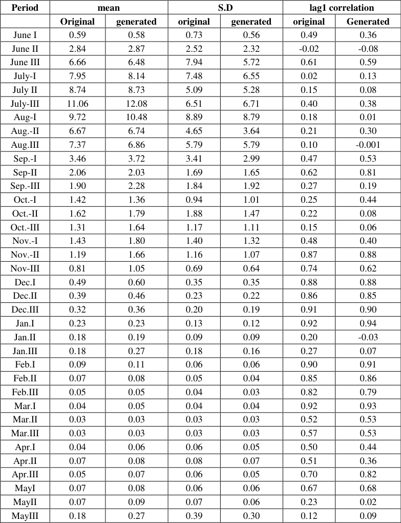 Table 2
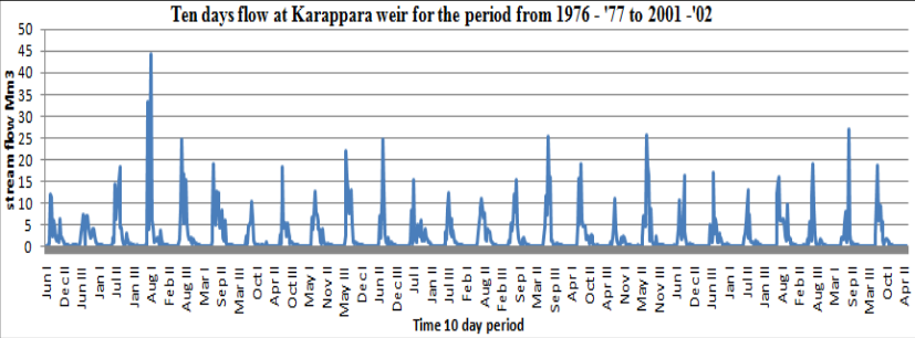 Figure 2
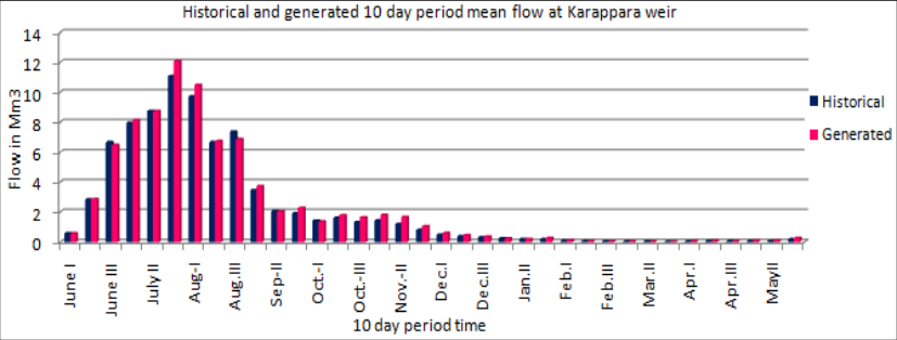 Figure 3
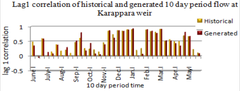 Figure 4
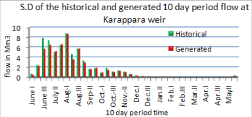 Figure 5
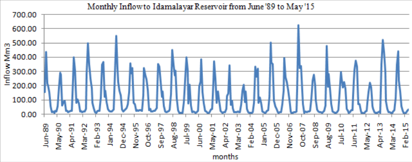 Figure 6
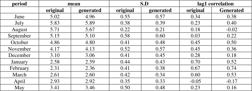 Table 3
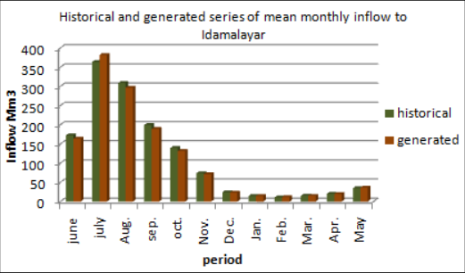 Figure 7
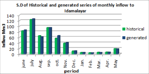 Figure 8
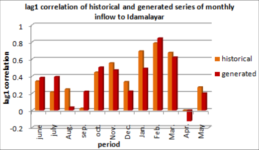 Figure 9
Introduction
The main impacts of climate change have been discussed globally over last two decades. It would affect agriculture in several ways. As far as water resources are concerned a warmer climate would accelerate the hydrological cycle and it can alter the intensity and timing of rainfall. Global warming and the resulted decline in rainfall may reduce net recharge and can affect ground water levels. Decrease in winter precipitation would reduce the total seasonal precipitation and can impose greater water stress. At the same time, soil erosion would be at a greater rate with increased rainfall amounts [1] . In this climate change scenario, distribution of water for agricultural purposes is a complicated issue and its management is generally affected by social, environmental and political factors [2] . Surplus water during rainy seasons can be stored in reservoirs and can be utilised for irrigation in drought periods. Prevention of floods can also be ensured. So a well organised operation of reservoir system is important for getting maximum net benefit from the available water resource. It will regulate inflows and provide outflows in a regular rate according to demand. Generally water management involves the supply and distribution of the right amount of water at the right time to the right place so that the agricultural, industrial and commercial activities and other day to day domestic needs of the society are satisfied. A serious constraint in this regard is the shortage of reservoir water. For a precise estimate of reservoir yield, simulation models need to be developed. Hence a study was carried out to develop stochastic models to simulate stream flow as well as reservoir inflow using the long term observed data and to compare the generated flow with the observed values and consequently to anticipate future flows with reliability. In general reservoir simulation models may be used directly to forecast the performance of a new reservoir or to model the historical behaviour of an existing reservoir [3] . Forecasts are made for a variety of operating conditions through the history matched model. Economic models are combined with these models to make decisions concerning the regular operations of the reservoir. The expected performance of the system can be evaluated for a set of given design and policy parameters. Based on given operating rules, the performance of the system for the next 50 or 100 years can be simulated. Determining the sequence of annual operations of irrigation and hydropower, the benefits derived out of it can be estimated. The sequential nature of the reservoir management decisions, together with the inherent randomness of natural water inflows direct us to use Markov decision processes for modelling reservoir management problems and their optimisation through stochastic dynamic programming [4] . Markov chain model was found to be useful as a predictive device for studying reservoir elevation of Shiroro Dam [5] . Synthetically generated sequences of the inflow are made use of for simulation of the reservoir operations. This branch of synthetic hydrology is well appreciated by Engineers and hydrologists because it can accommodate complex inflow models. The important elements involved in the modelling are the time unit of operation of the reservoir, the persistence of flows, the seasonality, the unit of volume, the release and finally the finiteness or otherwise of the reservoir [6] . A monthly time series model incorporating both seasonality and autocorrelation would be resulted if the time unit is a month. Markov processes with seasonality varying transition probabilities can be effectively used to model the persistence and the seasonality. The time unit can be selected as 10 days, 15 days or months according to the situation.
Location of the Study
The study was conducted to simulate reservoir inflow of Idamalyar Dam (10 0 13' 18" N 76 0 42' 21" E). It is a multipurpose concrete gravity Dam built across Idamalayar river, a tributary of Periyar river in Kerala. It originates in the Anamala hills at about 2500m above sea level. It has an annual rainfall of 6000mm and inflow of 5539Mm 3 . In addition, the storage is supplemented with water let from Nirar under interstate agreement and a portion of the excess water from the Poringalkuth reservoir of Chalakudy river. The water stored in the reservoir is used for generating electricity at the 75MW power station and the tail water is led to the Idamalayar river itself and collected at Bhoothathankettu barrage of Periyar Valley Irrigation Project. The irrigation benefits covers an area of 14394 hectares of agricultural land. The cultivable command area is 13209 hectares. The next location of study was the Karappara river near Nelliampathy in Palakkad District of Kerala. It is a tributary of Chalakudy river having a catchment area of 47.695km 2 for the gauging weir. Karappara-Kuriarkutty multi-purpose project for power generation and irrigation in the Chittur taluk, in Palakkad district which experiences severe shortage of water and power was proposed years ago.
Data and Methodology
Daily data on Idamalayar Reservoir inflow for a period from 1989 june -2015 May and the daily stream flow at Karappara gauging weir for a period from June '76 to May 2002 were used for the study. The main principle behind data generation in hydrology is that there is a statistical regularity of the hydrologic processes unless major changes occur. Information collected from the historical periods are used to make an assessment of how the process is likely to behave in the future and using this principle, data for the future is generated. The essential information content, in terms of probability, general stochastic behaviour of the process and statistical parameters are captured. Using these informations of the past data, future sequence of observations are generated. It is always better to base the future decisions upon several sequences rather than basing on a single sequence to avoid the risk of occurrence of extreme events like floods, droughts etc. All the parameters of the historical data would be extended or preserved so that the several sequences generated would follow the same distribution as that of the past.
As far as hydrologic processes are concerned, there is a persistence in nature. That means there is a tendency of flows to follow the trend of immediate past. The generating models reproduce the statistical distribution and persistence of historical flows and it will have the same mean, S.D and lag1 correlation as that of the historical data.
Data generation through first order Markov processstationary Data
If large time steps like annual time steps are taken neglecting periodicities, then stationary Markov process can be employed as Xt +1 = μx + ρ1 (Xt -μx) + €t+1 Xt +1 is the generated value for the time period t+1, μx is the long term observed mean of the process, ρ1 is the lag1 correlation of Xt +1 with Xt, € ≈ N(0, ⌐e 2 ). This model is stationary with respect to mean and variance. A sequence is to be generated with the same mean μx and variance ⌐x 2 € will have a mean 0. But to maintain the same variance ⌐x 2 for the process, properties of €t+1 are important.
Therefore ⌐e 2 = ⌐x 2 (1-ρ1 2 ) ie the variance of €t+1 would be ⌐e 2 = ⌐x 2 (1-ρ1 2 ) If Xt follows normal distribution with mean μx and variance ⌐x 2 and € should also be normally distributed with mean 0 and variance ⌐e 2 . Let a new variable Ut be introduced which follows N (0, 1), then Ut ⌐e ie Ut ⌐x √ (1-ρ1 2 ) is N (0, ⌐e 2 ). Thus it can be ensured that the random component has 0 mean and variance ⌐e 2 . Introducing a standard normal deviate Ut+1, the first order Markov model can be written as Xt +1 = μx + ρ1 (Xt-μx) + Ut+1 ⌐x √ (1-ρ1 2 ). Ut+1 follows standard normal distribution with mean 0 and variance 1. By using such a random number it can be ensured that the error component will have 0 mean and constant variance ⌐e 2 . The model would be stationary because the same value of mean and S.D is used to generate different values. The assumptions made to apply this model is that (1) the process Xt follows normal distribution with mean μx and variance ⌐x 2 and (2) the process is stationary in mean, S.D and lag1 correlation.
To start the generation procedure, first the moments viz; mean, S.D and lag1 correlation of the historical data are found out. To generate x2 from x1 using the model, x1 is initially assumed to be μx so that the second term in the model will immediately be zero. The standard normal deviates Ut+1 are straight away taken from the statistical tables or inbuilt programs. Once x2 is generated it is used to generate x3. Each time Xt and Ut+1 are changed in the model but all other parameters remain constant. Since the process was started by assuming Xt as μx, the first 100 or 150 values are to be discarded to do away with this effect. By changing the set of random numbers of standard normal deviate, several number of sequences can be generated. In all these sequences first few values are discarded to make it free from the effect of the initial value assumed to start the process. Since standard normal deviates ranges from -3 to +3, practically, the generated values may contain negative numbers. In such cases retain the negative number as such to generate the next number but in real applications it is taken as zero as the variables in hydrology such as stream flow, rainfall etc. will not assume negative values.
Data Generation through first order Markov Model with Non-Stationarity
In the first order stationary Markov model it is assumed that the mean, S.D and lag1 correlation should be the same for the historical and generated data. But when hydrological time series is considered they exhibit non stationarity especially when monthly data such as stream flow are considered. In this case the mean, S.D and lag1 correlation will significantly different from one month to another. So it is essential to incorporate these type of variations or non stationarity of the moments in the model. Relaxing the requirements of the first order stationary Markov model usually used for annual flows, seasonal models can be introduced in which the seasons can be either months, or any intra period or intra year variation. There may be periodicities existing in the data. The stream flow during a period may be correlated with a value in the previous periods and so on. In situations where there is a periodicity, it introduces non stationarity in the data. The periodicities would affect not only the mean and S.D but lag1 correlation also all of which appear in the Markov model. In the stationary Markov model, nonstationarity is introduced in the mean, S.D and lag1 correlation by taking one new index xi, j+1 where i is the year and j is the month. First order Markov model with non-stationarity, for data generation is given by where ρj is the serial correlation between flows of jth month and j+1 th month, ti, j+1 ~ N(0,1). Instead of the stationary mean μx, mean of a particular season for which data is generated is expressed as μj+1, ρj is the lag1 correlation between month j and j+1, ⌐ j indicating S.D for the particular month, ti, j+1 is drawn from N(0,1) ie random variables following standard normal distribution. To generate the values, first, μx, ⌐ j and ρj are estimated, then start with an assumed initial value and a value for the (j+1) th month is generated and so on.
Results and Discussion
The first order stationary Markov model as well as the model addressing the non stationarity are demonstrated using the data pertaining to Karappara stream flow and Idamalayar Reservoir Inflow. They were found to be very useful in modelling annual stream flows and reservoir inflows. These types of models can be effectively used in hydrological designing to fix the capacity of a reservoir, simulation of the performance of a reservoir etc. by using several sequences of generated data.
Simulation of Karappara Stream flow
The mean annual flow at Karappara weir was 79.42Mm 3 with a S.D of 26.81Mm 3 and lag1 correlation of 0.26. The yearly series of stream flow was found to follow normal distribution. The seasonal first order Markov model can accommodate shorter period flows such as 10 day period, weekly etc. to simulate data. But when the model is applied to very short periods like less than 10, the assumption of normality of the data may be violated. When 10 day period is used, the year is divided into 36 time intervals. The time series of the 10 day period flow at Karappara weir is depicted in Fig. (2). Each month was divided into three viz; juneI, juneII, juneIII etc.. For each of these periods, the moments viz; mean, S.D and lag1 correlation were found out. The simulated values were then derived using First order Markov model. First hundred values generated were discarded and the characteristics of the next 50 values generated are summarised in Table2. The moments of the historical and generated series compared well. The adequacy of the fitted model is shown in Fig. 3, Fig. 4 and Fig. 5.
| Period | mean | — | S.D | — | lag1 correlation | — |
|---|---|---|---|---|---|---|
| Original | generated | original | generated | original | Generated | |
| June I | 0.59 | 0.58 | 0.73 | 0.56 | 0.49 | 0.36 |
| June II | 2.84 | 2.87 | 2.52 | 2.32 | -0.02 | -0.08 |
| June III | 6.66 | 6.48 | 7.94 | 5.72 | 0.61 | 0.59 |
| July-I | 7.95 | 8.14 | 7.48 | 6.55 | 0.02 | 0.13 |
| July II | 8.74 | 8.73 | 5.09 | 5.28 | 0.15 | 0.08 |
| July-III | 11.06 | 12.08 | 6.51 | 6.71 | 0.40 | 0.38 |
| Aug-I | 9.72 | 10.48 | 8.89 | 8.79 | 0.18 | 0.01 |
| Aug.-II | 6.67 | 6.74 | 4.65 | 3.64 | 0.21 | 0.30 |
| Aug.III | 7.37 | 6.86 | 5.79 | 5.79 | 0.10 | -0.001 |
| Sep.-I | 3.46 | 3.72 | 3.41 | 2.99 | 0.47 | 0.53 |
| Sep-II | 2.06 | 2.03 | 1.69 | 1.65 | 0.62 | 0.81 |
| Sep.-III | 1.90 | 2.28 | 1.84 | 1.92 | 0.27 | 0.19 |
| Oct.-I | 1.42 | 1.36 | 0.94 | 1.01 | 0.25 | 0.44 |
| Oct.-II | 1.62 | 1.79 | 1.88 | 1.47 | 0.22 | 0.08 |
| Oct.-III | 1.31 | 1.64 | 1.17 | 1.11 | 0.15 | 0.06 |
| Nov.-I | 1.43 | 1.80 | 1.40 | 1.32 | 0.48 | 0.40 |
| Nov.-II | 1.19 | 1.66 | 1.16 | 1.07 | 0.87 | 0.88 |
| Nov-III | 0.81 | 1.05 | 0.69 | 0.64 | 0.74 | 0.62 |
| Dec.I | 0.49 | 0.60 | 0.35 | 0.35 | 0.88 | 0.88 |
| Dec.II | 0.39 | 0.46 | 0.23 | 0.22 | 0.86 | 0.85 |
| Dec.III | 0.32 | 0.36 | 0.20 | 0.19 | 0.91 | 0.90 |
| Jan.I | 0.23 | 0.23 | 0.13 | 0.12 | 0.92 | 0.94 |
| Jan.II | 0.18 | 0.19 | 0.09 | 0.09 | 0.20 | -0.03 |
| Jan.III | 0.18 | 0.27 | 0.18 | 0.16 | 0.27 | 0.07 |
| Feb.I | 0.09 | 0.11 | 0.06 | 0.06 | 0.90 | 0.91 |
| Feb.II | 0.07 | 0.08 | 0.05 | 0.04 | 0.85 | 0.86 |
| Feb.III | 0.05 | 0.05 | 0.04 | 0.03 | 0.82 | 0.79 |
| Mar.I | 0.04 | 0.05 | 0.04 | 0.04 | 0.92 | 0.93 |
| Mar.II | 0.03 | 0.03 | 0.03 | 0.03 | 0.52 | 0.53 |
| Mar.III | 0.03 | 0.03 | 0.03 | 0.03 | 0.57 | 0.53 |
| Apr.I | 0.04 | 0.06 | 0.06 | 0.05 | 0.50 | 0.44 |
| Apr.II | 0.07 | 0.08 | 0.08 | 0.07 | 0.51 | 0.36 |
| Apr.III | 0.05 | 0.07 | 0.06 | 0.05 | 0.70 | 0.82 |
| MayI | 0.07 | 0.08 | 0.06 | 0.06 | 0.67 | 0.68 |
| MayII | 0.07 | 0.09 | 0.07 | 0.06 | 0.23 | 0.02 |
| MayIII | 0.18 | 0.27 | 0.39 | 0.30 | 0.12 | 0.09 |
Table text extracted from the original PDF; superscript letters are shown inline. The original table image is below.
View original table image
Acknowledgement
The Authors are grateful to Prof. Dr. P.P. Mujumdar, IISc Bangalore for the technical help received on the topic through his series of Lectures on Time Series Analysis. The authors also express sincere gratitude to Kerala state Electricity Board Ltd. for providing the data for the study.
Figures and tables from the paper
| Annual flow | Mean (Mm3) | S.D (Mm3) | Lag1 correlation |
|---|---|---|---|
| Historical data | 79.42 | 26.81 | 0.26 |
| Generated data | 80.37 | 25.20 | 0.35 |
Table text extracted from the original PDF; superscript letters are shown inline. The original table image is below.
View original table image
| period | mean | — | S.D | — | lag1 correlation | — |
|---|---|---|---|---|---|---|
| original | generated | original | generated | original | Generated | |
| June | 5.02 | 4.96 | 0.55 | 0.57 | 0.34 | 0.38 |
| July | 5.83 | 5.89 | 0.38 | 0.39 | 0.23 | 0.40 |
| August | 5.71 | 5.67 | 0.22 | 0.21 | 0.18 | -0.02 |
| September | 5.15 | 5.10 | 0.58 | 0.60 | 0.03 | 0.22 |
| October | 4.86 | 4.80 | 0.41 | 0.48 | 0.45 | 0.50 |
| November | 4.17 | 4.13 | 0.52 | 0.57 | 0.45 | 0.36 |
| December | 3.10 | 3.06 | 0.41 | 0.45 | 0.28 | 0.18 |
| January | 2.58 | 2.59 | 0.44 | 0.43 | 0.70 | 0.52 |
| February | 2.31 | 2.36 | 0.41 | 0.38 | 0.67 | 0.74 |
| March | 2.61 | 2.60 | 0.42 | 0.34 | 0.60 | 0.53 |
| April | 2.93 | 2.92 | 0.35 | 0.33 | -0.05 | -0.17 |
| May | 3.41 | 3.46 | 0.50 | 0.48 | 0.23 | 0.16 |
Table text extracted from the original PDF; superscript letters are shown inline. The original table image is below.
View original table image
References
5 in the original paper- Goutam KS. Climate change -man and environment. ISBN: 9788170357711. Daya publishing House, New Delhi. 2012, 290.
- Ward MN, Brown CM, Baroang KM, Kaheil YH. Reservoir performance and dynamic management under plausible assumptions of future climate over seasons to decades. Climate change. 2013; 118(2):307-320.
- Lamond BF, Boukhtouta A. Water reservoir applications of Markov decision processes in Feinberg E.A, Shwartz A (eds). Handbook of Markov decision processes. International series in operations research and management science, Springer, Boston M.A. 2002; 40:537-558.
- Abubakar UY, Hakimi D, Mohammed A, Lawal A. A non-stationary transition probabilities for a reservoir elevation of hydroelectric power Dam. Journal of Mathematics. 2014; 10(3):39-44.
- Phatarford RM. Riverflow and reservoir storage models. Mathematical and computer modelling. 1989; 12(9):1057-77.