
Research article · 2019 · Full text
International Journal of Statistics and Applied MathematicsEffect of sinusoidal thermal boundary condition on unsteady Magnetohydrodynamics convection in a square enclosure filled with Fe3O4-water Ferrofluid
Volume 4(6) · Pages 111–127
Research areasCharacterization and Applications of Magnetic NanoparticlesGeomagnetism and Paleomagnetism StudiesNanofluid Flow and Heat Transfer
Abstract
Author-writtenFerrofluid convective heat transfer in a square cavity with sinusoidal temperature boundary condition at the bottom wall under the influence of magneto hydrodynamics effect was investigated numerically in the present study. Top wall is maintained at comparatively low temperature and Vertical walls are assumed to be adiabatic. The working fluid is Fe3O4-water nanofluid. Single phase model is used to estimate the behavior of ferrofluid and the Maxwell-Garnet model is used for modeling the effective thermal conductivity and viscosity for the ferrofluid. The Galerkin weighted residual method of finite element analysis is implemented to discretize the governing equations. The analysis has been carried out for solid volume fraction (φ = 0- 0.1) and the Hartmann number (Ha = 0-20) for two values of Rayleigh number (Ra = 105, 106) with respect to dimensionless time (τ = 0.1, 1.0). The results are presented both in terms of streamlines, isotherms and Local Nusselt number through the active thermal wall for different combinations of the governing parameters. The results indicate that both the flow and the thermal fields strongly depend on the above-mentioned parameters. The computational results also indicate that the Local Nusselt number at the heated wall for different time are depending on the aforementioned parameters. The results in terms of local Nusselt number are also shown in tabular form. The present investigation lays down a solid foundation for the investigation of time-varying sinusoidal boundary conditions in MHD convection.
Summary
Source-checkedPlain-language reading of the full paper, prepared with AI and checked against the text. Each point links to the authors' own words.
Why it matters
- Nanofluids are used to improve heat transfer, and ferrofluids are a specific type of nanofluid that can be controlled using magnetic fields. View evidence ↗
- Ferrofluids have practical applications in several engineering fields, including aerospace, bioengineering, and electronic packaging. View evidence ↗
- Many heat-transfer problems, particularly in electronics, involve both strong magnetic fields and sinusoidal heating patterns. View evidence ↗
The question
- The study aims to investigate how a magnetic source affects the hydrothermal behavior of a nanofluid within a cavity that has a sinusoidally heated wall. View evidence ↗
What they did
- The researchers used an Fe3O4-water nanofluid, modeled as a single-phase continuum, with the Maxwell-Garnet model used to determine effective viscosity and thermal conductivity. View evidence ↗
- The governing equations were discretized using the Galerkin weighted residual method of finite element analysis. View evidence ↗
What they found
- At a dimensionless time of 0.1, the flow creates four opposing vortices: two large ones in the middle of the bottom wall and two small ones at the corners. View evidence ↗
- Heat transfer is enhanced when both the nanoparticle volume fraction and the thermal Rayleigh number are increased. View evidence ↗
What it means
- The authors conclude that the magnetic field can serve as a control parameter because increasing the Hartmann number reduces flow velocity, strength, and heat transfer. View evidence ↗
- The study concludes that both flow strength and heat transfer increase as the Rayleigh number increases across all tested cases. View evidence ↗
Visual summary
2 visualsIllustrations explain the paper; charts are replotted from the paper's own table values.
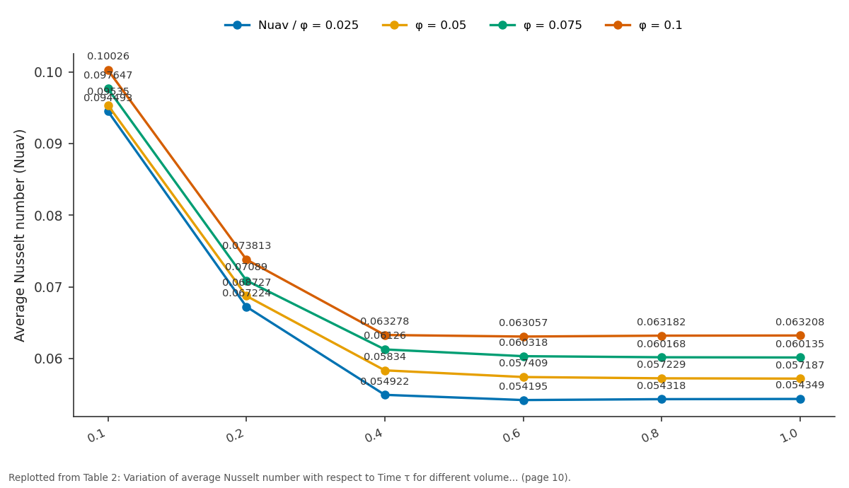
Nuav / φ = 0.025 and φ = 0.05 and more: 0.1 vs 0.2 vs 0.4 vs 0.6 vs 0.8
Replotted from Table 2 (page 10) of the original paper. Every bar is the paper's own table value.
View source evidence ↗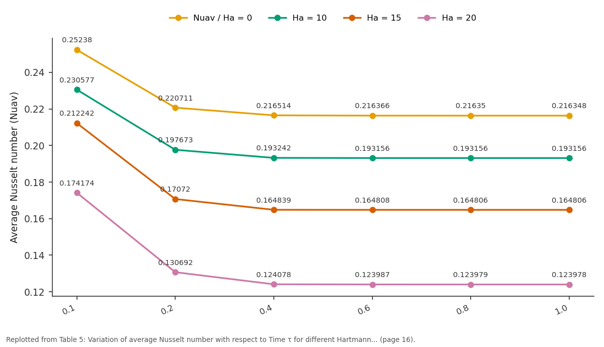
Nuav / Ha = 0 and Ha = 10 and more: 0.1 vs 0.2 vs 0.4 vs 0.6 vs 0.8
Replotted from Table 5 (page 16) of the original paper. Every bar is the paper's own table value.
View source evidence ↗Figures & tables
From the original paper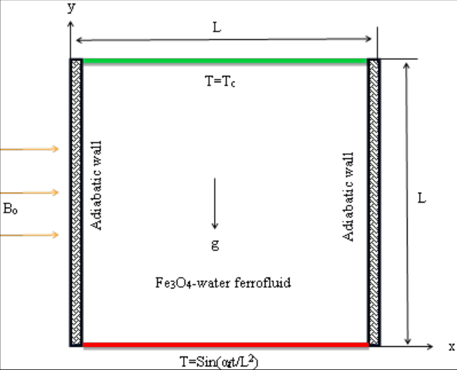 Figure 1Page 2
 Table 1Page 4
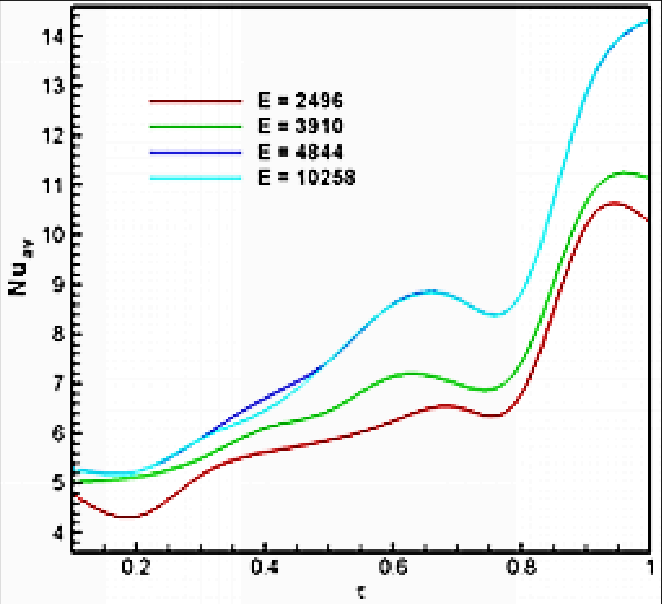 Figure 2Page 5
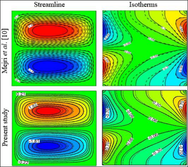 Figure 3Page 5
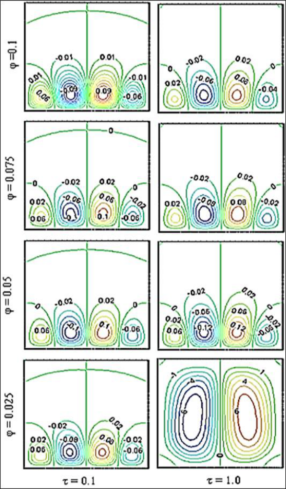 Figure 4Page 6
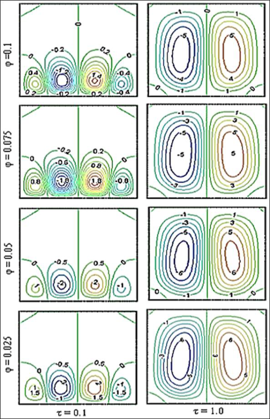 Figure 5Page 7
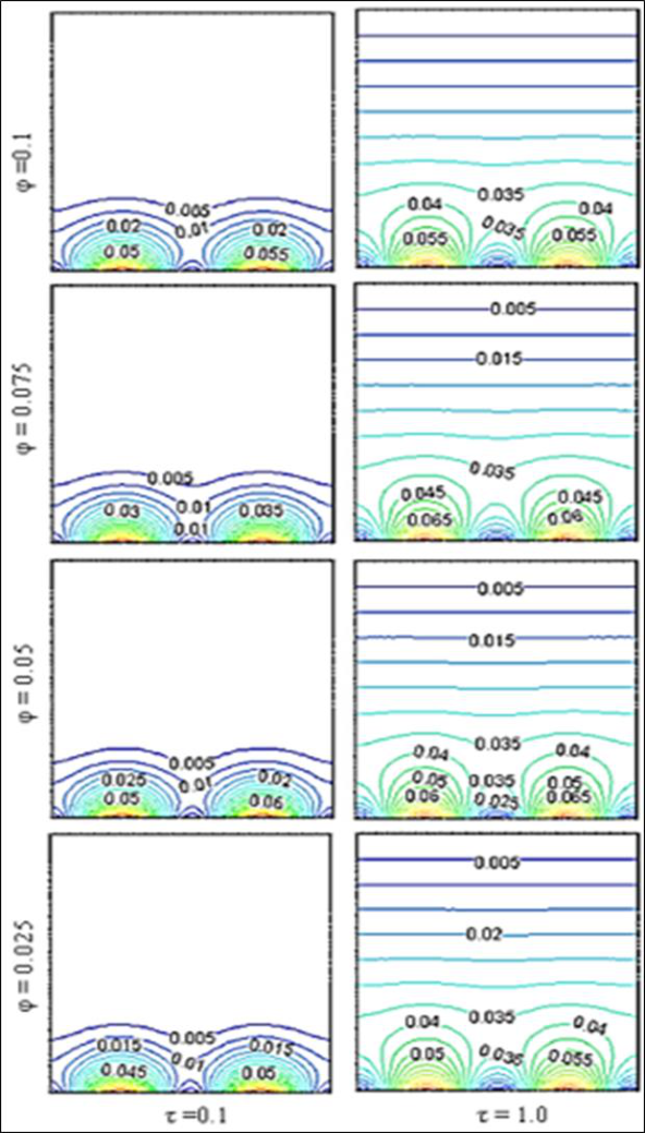 Figure 6Page 8
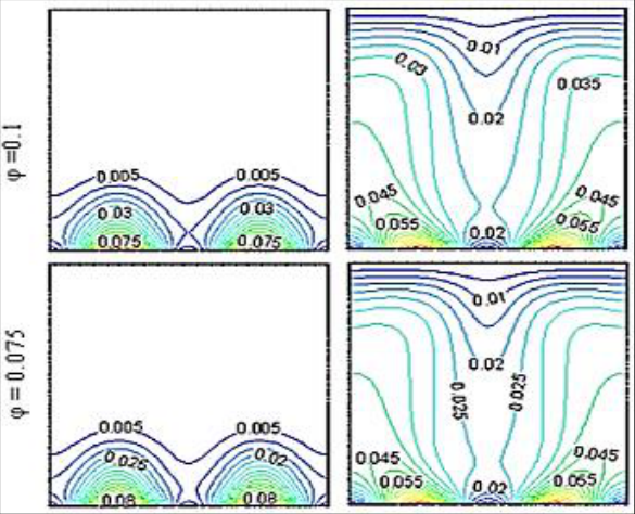 Figure 6Page 8
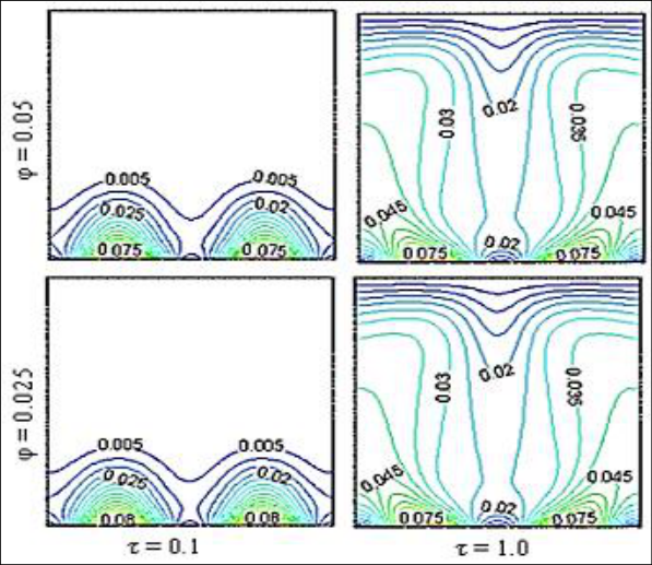 Figure 7Page 9
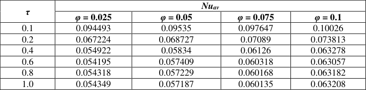 Table 2Page 10
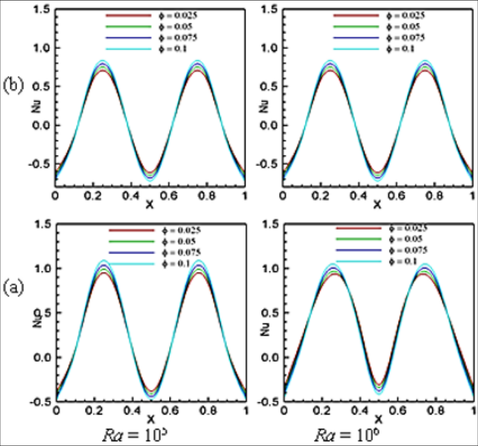 Figure 8Page 10
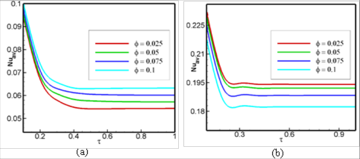 Figure 9Page 10
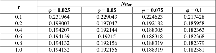 Table 3Page 11
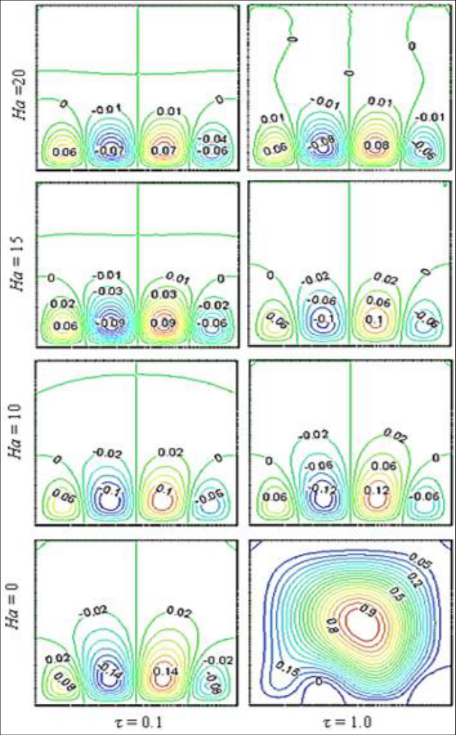 Figure 10Page 11
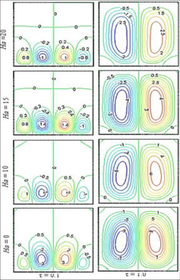 Figure 11Page 12
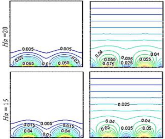 Figure 11Page 12
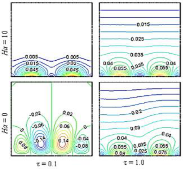 Figure 12Page 13
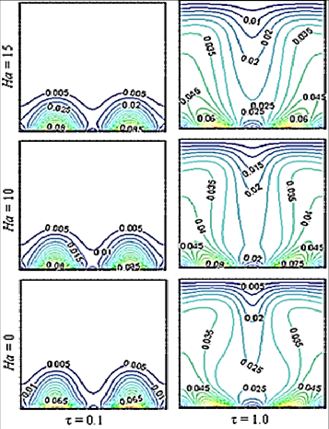 Figure 13Page 14
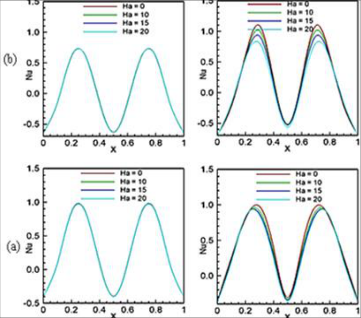 Figure 14Page 15
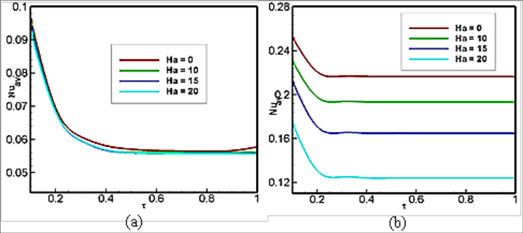 Figure 15Page 15
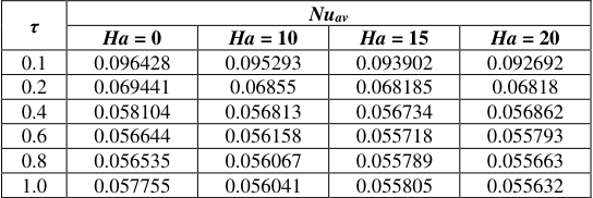 Table 4Page 16
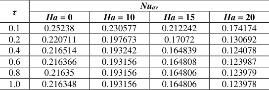 Table 5Page 16
Introduction
Innovative kinds of fluid were required to reach more efficient performance in new days. Nanofluid was proposed as innovative way to enhance heat transfer. Among a variety of nanofluids, those that respond to magnetic fields are called ferrofluid. Magnetic fields propel ferro particles by applying magnetic force and affect their technology.
Investigations on the effects of nanofluids and ferrofluid under different geometries and configurations are rich and have attracted many researchers to study their role in the field of heat transfer. As a magnetic nanofluid, ferrofluid, are used in various fields such as electronic packing, mechanical engineering, thermal engineering, aerospace and bioengineering. Nanofluids have been simulated in a lot of studies in different aspects. Comprehensive literature survey concerned with this subject is given [1-2].
Magnetic field effects in convection can be altered by adding nano-sized particles to the base fluid, which changes both the thermal and electrical conductivity of the fluid [3, 4]. The inclusion of a very small number of nanoparticles to the base fluid may result in significant enhancement of heat transfer, and various factors affect the amount of enhancement, such as size, shape and type of the particles. Nanofluid technology has been successfully implemented in various thermal engineering applications [5, 6]. In recent year Selime fendigil et al. [7] investigated forced convection of Fe3O4-water nanofluid in a bifurcating channel under the effect of variable magnetic field.
Wu et al. [8] studied natural convection for porous rectangular cavity having sinusoidal temperature distribution in both side walls and they found a sinusoidal thermal boundary condition enhances the heat transfer significantly. Recently, Rahman et al. [9] studied unsteady heat transfer in a square cavity filled Maths 2019; 4(6): 111-127 Eare Md. Morshed Alam Department of Mathematics, Jahangirnagar University, Savar, Dhaka, Bangladesh Sumona Huq Department of Mathematics, Bangladesh University of Engineering and Technology BUET, Dhaka, Bangladesh Md. Sharif Uddin Department of Mathematics, Jahangirnagar University, Savar, Dhaka, Bangladesh MM Rahman Department of Mathematics, Bangladesh University of Engineering and Technology BUET, Dhaka, Bangladesh MM Rahman Department of Mathematics, Bangladesh University of Engineering and Technology BUET, Dhaka, Bangladesh http://www.mathsjournal.com with CNT–water nanofluid having non-isothermal bottom heater.
They concluded the nanofluid allows for an optimum enhancement of heat transfer. In general, heating can be classified as isothermal or non-isothermal. Mejri et al. [10] studied MHD natural convection in a nanofluid-filled open cavity with a sinusoidal boundary condition and they reported incrementing Ha decreases the heat transfer for the nanofluid. Jue [11] analyzed combined thermal and magnetic convection in a ferrofluid filled square cavity using a semi-implicit finite-element method.
For the cavity, the side walls are kept at different temperatures and the position of magnetic field was at the bottom. The author concluded that a suitable location and orientation of the magnetic field is useful for enhancing heat transfer in practical applications. Effect of sine-squared thermal boundary condition on augmentation of heat transfer in a triangular solar collector filled with different nanofluids and semi-circular enclosure with ferrofluid investigated numerically and statistically by Rahman et al. [12, 13]. Rabbi et al. [14] recently investigated mixed convection in ferrofluid filled lid driven cavity in different heater configuration and found that at higher Ri and lower Ha, semi-circular notched cavity shows significantly better (more than 30%) heat transfer rate.
In the numerical study by Sheikholeslami et al. [15], forced convection of magnetic nanofluid in a lid-driven semi annulus was examined with CVFEM. The average Nusselt number was observed to increase with nanoparticle volume fraction while the heat transfer enhancement was found to decrease with higher values of Reynolds number and lower values of Hartmann number. Khanafer et al. [16] tried to simulate numerically the flow and heat transfer of Cu-water nanofluid using the finite–volume (FV) approach. In their work, four different methods for nanofluid treatment were examined and the results were compared to the experimental data.
Sheikholeslami and Ganji [17] analyzed ferrofluid flow in a semi annulus with an external magnetic field by using control volume based finite element method (CVFEM) considering both ferro-dynamics and magneto hydrodynamics. Magnetic number was found to influence the heat transfer differently depending on the Rayleigh number while both increasing nanoparticle volume fraction and decreasing Hartmann number were found to enhance the heat transfer rate. A careful review of the above existing literature reveals that there is a lack of fundamental information. The main purpose of this study was to investigate impact of magnetic source on hydrothermal behavior of nanofluid in a cavity with sinusoidal type heating wall.
Effects of Rayleigh and Hartmann numbers, volume fraction of Fe3O4 on hydrothermal treatment are considered and their effect on heat transfer is analyzed by following their dimensionless-time evolution. The present investigation can be applied to design more realistic heat transfer equipment consider as sinusoidal-type time-dependent heating. 2. Problem formulation 2.1 Physical model The physical model considered here as shown in Fig. 1, along with the important geometric parameters. We consider a two- dimensional square enclosure having length and width L.
As seen from the schematic view, the top wall of the cavity is kept at a low temperature Tc and the bottom wall of the enclosure is heated and its temperature at the boundary varies sinusoidally with time. Whereas on the left and right-vertical walls the thermal conditions are adiabatic. We considered Fe3O4-water nanofluid and assumed incompressible, Newtonian fluid. Thermo physical properties of water and Fe3O4 nano particles are given in Table 1.
| — | cp (Jkg−1K−1) | Ρ (kgm−3) | K (Wm−1K−1) | Β (K−1) | Σ (Siemens m−1) |
|---|---|---|---|---|---|
| Water | 4179 | 997.1 | 0.613 | 2.1 × 10⁻⁴ | 0.05 |
| Fe3O4 | 670 | 5200 | 6 | 1.3 × 10⁻⁵ | 25,000 |
Table text extracted from the original PDF; superscript letters are shown inline. The original table image is below.
View original table image
The gravity acts in the negative y-direction. The radiation, pressure work and viscous dissipation are assumed to be negligible. For mathematical modeling, the fluid is assumed to be of single-phase continuum. Fig 1: Schematic diagram of the physical model and boundary along with the coordinate system The flow is considered to be unsteady, two dimensional and laminar.
The viscous dissipation and radiation heat transfer are also neglected. A magnetic field with magnetic flux density Bo is applied horizontally on the left of the enclosure. Given boundary conditions describing time-dependent sinusoidally heating, the bottom wall steadily heats as time intervenes. In practice, heating goes up sinusoidally in many heat-transfer problems.
In electronic heat transfer, there is also the presence of a strong magnetic field. To study the time-dependent behavior of such heat transfers, the following analysis is beneficial. http://www.mathsjournal.com 2.2 Mathematical modeling 2.2.1 Governing equation The governing equations of the problem specification are conservation of mass, momentum and energy equations. The Boussinesq proximation is employedfor the density variation of the fluid. Under these assumptions, the governing equations for the unsteady, two-dimensional, laminar and incompressible nanofluid MHD flow in dimensionless form can be written as follows: 0 U V X Y (1) 2 2 ff 2 2 ff f U U U P U U U V X Y X X Y (2) V V ff ff f ff Ra Ha V ff f ff f ff f 2 2 ( ) 2 Pr Pr 2 2 V V V P U V X Y Y X Y (3) 2 2 ff 2 2 U V X Y f X Y (4) Where U, V, P, and θ are the dimensionless velocity, pressure and temperature respectively.
Here, subscripts ‘ff’ and ‘f’ refer to ferrofluid and base fluid respectively. The effective thermo-physical properties of ferrofluids are defined by using the following formula: The density of ferrofluid, which is assumed to be constant, can be expressed as 1 . ff f s (5) The effective thermal diffusivity of the ferrofluid can be modeled as k ff ff c p ff (6) Where the heat capacitance of the ferrofluid ff(pcρ) is given by 1 . p p p ff f s c c c (7) In addition, the thermal expansion coefficient ffβ of the ferrofluid follows from 1 . ff f s (8) (9) Moreover, the dynamic viscosity μffof the ferrofluid can be expressed using the Brinkman model [18], f ff 2.5 . 1 The effective thermal conductivity of the ferrofluid can be described using the Maxwell–Garnet model [19], 2 2 k k k k k s f f s ff k k k k k 2 f s f f s (10) And the effective electrical conductivity of the ferrofluid can be described using the Maxwell–Garnet model [19]. s f ff 3 1 1 . 2 1 f s f s f (11) http://www.mathsjournal.com 2.2.2 Boundary conditions The transformed initial and boundary conditions are: τ = 0, At entire domain: 0, 0 U V τ >1, at top wall: 0, 0, 0 U V At left and right wall: 0, 0, 0 U V N At the bottom wall: 0, U V Sin Where N is the non-dimensional distances either along X or Y direction acting normal to the surface. The governing equations, initial and boundary conditions are transformed into dimensionless forms using the following dimensionless variables as: 2 2 2 , , , , , , . f f c p gy L t T T x y uL vL X Y U V P L L L T T f f ff f h c The dimensionless parameters in the above equations, where Ra is the Rayleigh number, Pr is the Prandtl number and Ha is the Hartmannnumber are defined as: 3 g L T T Ra Pr Ha B L respectively. , , f h c f f o f f f f The local Nu on the heat source surface can be expressed as . ff L k Nu k Y f 1 The average Nusselt evaluated along the heat source can be expressed as av 0 . ff k Nu dX k Y f The non-dimensional stream function is defined as: , U V y x . 2.3 Properties of ferrofluid The thermo physical properties of the Fe3O4 ferromagnetic particle and water (base fluid) is presented in Table 1. Table 1: Thermo physical properties of water and Fe3O4 nanoparticle cp (Jkg−1K−1) Ρ (kgm−3) K (Wm−1K−1) Β (K−1) Σ (Siemens m−1) Water 4179 997.1 0.613 2.1 × 10⁻⁴ 0.05 Fe3O4 670 5200 6 1.3 × 10⁻⁵ 25,000 3.
Numerical Methodology 3.1 Numerical schemes Galerkin weighted residual finite element method is used to complete discretization process of the system of nonlinear partial differential equations, (Eqs. (1)-(4)), subject to their corresponding initial and boundary conditions. Details of the process are accessible Zienkiewicz and Taylor [20]. The entire domain is first discretized into several triangular elements. The quadratic triangular element has been used to develop the finite element equations.
For the velocities and temperature all the six nodes are used and for the pressure only the corner nodes are used. Substitution of the obtained approximations into the system of the governing equations and boundary conditions yield a residual for each of the conservation equations. These residuals are reduced to zero in a weighted sense over each element volume using the Galerkin weighted residual method. Then finally we use Triangular Factorization method to solve these linear equations.
The iteration has been done till the solution becomes convergent|Гm+1 – Гm| ≤ 10–6 where m is the number of iteration and Γ is the general dependent variable. 3.2 Grid test Preliminary results are obtained to inspect the field variables grid independency solutions. Test for the accuracy of grid fineness has been carried out to find out the optimum grid number. Figure 2 shows the grid test result for Ra= 105, Ha= 10, and a solid volume fraction of 10%. The average Nu is plotted against dimensionless time τ.
From the figure, it is clear that average Nu varies significantly for 4844elements. After we reached a grid having 10258 elements, there is no significant variation in the average Nu. Therefore, setting the number of elements to 4844 as our standard, this size of grid reduces the computational time and cost without hampering the accuracy of numerical results. http://www.mathsjournal.com Fig 2: Grid sensitivity test at = 0.04, Ha = 10 and Ra = 105 3.3. Code verification The code of this present investigation is verified with the previous numerical study of Mejri et al. [10] for square cavity filled with Al2O3-water nanofluid.
A comparison of the flow field and the thermal field between Mejri et al. [10] and present study for Ra = 5 × 10⁴, Ha = 50 and φ = 0 and 0.04. is presented in Fig. 3. This figure shows that agreement between them is good. Fig 3: Comparison of streamline and isotherm contours for Ra = 5 × 10⁴, Ha = 50 between numerical results by Mejri et al. [10] and present study
Results And Discussion
Primary objective of this numerical investigation is to discuss the effect of solid volume fraction and magnetic field is presented for unsteady convection. Fe3O4-water is considered as a single-phase ferrofluid; its solid volume fraction is varied from 2.5-10%. The value of Ra is fixed at 105 and 106 and four different Hartmann number (Ha) are chosen as 0, 10, 15 and 20. All the simulations are performed for dimensionless time τ=0.01 and 1.0.
In this section, the streamlines, isotherms, Local Nusselt number at the hot wall in the cavity are plotted with sinusoidally heated wall for different aforesaid parameters. http://www.mathsjournal.com 4.1. Effect of solid volume fraction The flow fields in terms of computed streamlines for the four representative values of the solid volume fraction φ (φ = 0.025, 0.05, 0.075 and 0.1), while Ha = 10, Ra = 105 with respect to time τ = 0.1 and 1.0 are shown in figure 4. For τ = 0.1, the streamline patterns are regular and four opposing vortices are created inside the cavity. Two large opposing vortices are created at the middle of the bottom wall of the cavity whereas the two small vortices are created at the two corners of the bottom wall.
This is quite obviously due to the sinusoidal time-dependent boundary condition. Incrementing the solid volume fraction does not show any significant effect for times τ = 0.1, although the regular streamline pattern is strong for φ=0.1. At τ= 1.0, two large counter rotating vortices are created inside the cavity for φ=0.025. Two major symmetric vortices oppose each other in the cavity.
Fluid rises up from the middle of the bottom wall and flows down along the two vertical walls, forming two symmetric rolls with clockwise and anticlockwise rotations inside the cavity. At this time τ =1.0, for other values of φ the streamline patterns are regular and four opposing vortices are created inside the cavity. Incrementing the solid volume fraction also does not show any significant effect for times τ = 1.0. The magnitude of the stream function is small signifying conduction dominant heat transfer within the cavity for the lower value of Ra = 105.
Near the bottom wall of the cavity, convection is isothermal and at a higher temperature than that near the top wall. As a result, strong convection occurs because of this temperature difference. The fluid is heated at the heated bottom wall, then pushed upwards by the buoyancy force, and finally returned after transferring heat to the cold top wall. This creates strong eddies, positioned in the bottom of the cavity.
Figure 5 illustrates the flow field for Ra = 106 for different solid volume fractions at τ = 0.1 and 1.0. For τ = 0.1, the streamline patterns are regular and four counter rotating vortices are created inside the cavity. Two large opposing vortices are created at the middle of the bottom wall of the cavity whereas the two small opposing vortices are created at two corners of the bottom wall. This is quite obviously due to the sinusoidal time-dependent boundary condition.
Fig 4: Effect of solid volume fraction on streamlines for the selected values of τ with Ha = 10 and Ra = 105 http://www.mathsjournal.com Fig 5: Effect of solid volume fraction on streamlines for the selected values of τ with Ha = 10 and Ra = 106 The magnitude of the stream functions is diminished slowly and the thickness of the layer of stream lines are increased for the incrementing values of φ. For τ = 1.0, two large symmetric counter rotating vortices are created inside the cavity for φ=0.025 which oppose each other in the cavity. Fluid rises up from the middle of the bottom wall and flows down along the two vertical walls, forming two symmetric rolls with clockwise and anticlockwise rotations inside the cavity. The magnitude of the stream functions remained same for φ=0.025 and φ=0.05 but reduced a little bit for other two incrementing values of φ.
It is seen that the streamlines for the four values of φ at τ = 1.0 appear to be almost identical. From Figs. 4 and 5, it is seen that the effect of Ra on streamlines is very significant. This may be due to the increased convection currents at the center due to increase in Rayleigh number and these convection currents push the heated fluid towards the side walls. With increasing Ra, the temperature difference between the bottom and top walls of the cavity increased.
With increasing Ra to 106, due to the time-dependent sinusoidal boundary condition, it takes a longer time to arrive at the steady state. The fluid inside the cavity then tries to increase the temperature of the cold wall. The solid volume fraction of the ferrofluid determines largely the flow pattern of the fluid at τ = 1.0. For τ = 1.0, the bottom wall is heated more than for τ = 0.1, and hence also causes a significant variation in the flow behavior between these two cases.
Figure 6 demonstrates the thermal field for different solid volume fractions of the ferrofluid for τ = 0.1 and 1.0. The figure provides the information about the influence of solid volume fraction on isotherms for the selected values of τ with Ha = 10 and Ra = 105. Two smooth, parabolic temperature distribution is observed for the lowest values of Ra = 105 on the bottom wall at τ = 0.1 which is separated by a small thermal layer. The two corners of the bottom wall are covered by a minor thermal line.
Also, the temperature distribution of the bottom wall is lower than that for τ = 1.0. Iso-thermal lines cover only the lower part of the enclosure. Thermal boundary layer thickness increases and iso thermal line become denser at the adjacent area of the bottom wall. The iso-thermal lines of the upper layers look like a sine wave and it flows on towards the two side walls.
So, heat is transferred by convection only in the lower part of the enclosure at initial time. This phenomenon can be explained by the fact that with smaller time intervals the fluid does not move under the lower buoyancy force available. Therefore, heat transfer does not occur between the fluid layers by convection in the upper portion of the enclosure. Therefore, the fluid is static-like and no fluid convection takes place a higher solid volume fraction of ferrofluid does not improve the degree of convection.
At τ = 1.0, two major thermal plumes formed at the bottom of the bottom wall which is separated by a minor thermal plume. Each of the corners of the bottom wall is also covered by a minor thermal plume. It indicates that heat is transferred by convection only in the lower part of the enclosure. http://www.mathsjournal.com Fig 6: Effect of solid volume fraction on isotherms for the selected values of τ with Ha = 10 and Ra = 105 http://www.mathsjournal.com Fig 7: Effect of solid volume fraction on isotherms for the selected values of τ with Ha = 10 and Ra = 106 Rest of the cavity is covered by isotherms parallel to each other indicating a conduction-dominated heat transfer at the rest of time for all aforesaid value of solid volume fraction. Incrementing the solid volume fraction also does not show any significant variation in the mode of heat transfer.
Figure 7 provides the information about the influence of solid volume fraction on isotherms for the selected values of τ with Ha = 10 and Ra = 106. For Ra = 106 and τ = 0.1, two smooth, parabolic temperature distribution are observed on the heater of the bottom wall which indicates that the heat transfer occurs by convection and it remains confined near the bottom only and heat transfer does not occur between the fluid layers by convection in the upper portion of the enclosure. The iso-thermal lines of the upper layers look like a sine wave and it flows on towards the two side walls. With increasing the value of φ, almost identical temperature distribution is observed at τ = 0.1.
At τ = 1.0 isotherms are covering most of the areas of the cavity which indicates convection heat transfer occurs in those areas. It is observed that at the end of process τ = 1.0 the symmetric patterns of isothermal lines indicate that heat goes upward from the sinusoidal heated bottom wall and falls on the two side walls equally and also observed that the thermal line near the upper wall is almost parallel to the top cold wall. It is seen that the temperature distribution for all selected values of φ at τ = 1.0 appear to be almost identical. From Figs. 6 and 7, it is seen that the effect of Ra on isotherm is very significant.
This may be due to the increased Ra, the temperature difference between the bottom and top walls of the cavity increased. With increasing Ra to 106, due to the time-dependent sinusoidal boundary condition, it becomes more nonlinear for all aforesaid value of ϕ due to strong buoyancy effect. Figure 8 gives the local Nu distribution for Ra = 105 and 106 at different dimensionless times and solid volume fractions. For τ = 0.01,no convection occurs at a very early stage.
For both Ra = 105 and Ra = 106, there is hardly any variation in the local Nu distribution at the heated bottom boundary. At the beginning local Nu is negative. This phenomenon is quite obvious as no fluid motion is established at this early stage of convection. After this time due to the effect of sinusoidal thermal boundary condition the Nusselt number will go up very quickly, it reaches a maximum value, then gradually decreases and it reaches a minimum near x=0.5.
For the remaining portion of the cavity a similar pattern of oscillation for the local Nu distribution is observed after this value of x. For this value of τ, the local Nu is higher for higher solid volume fraction at the point of maximum. On the other hand, the local Nu is lower for the higher solid volume fraction at the point of minimum. For τ = 0.5 in both the cases Ra = 105 and Ra = 106, there is no variation in the local Nu distribution except the fact that the extent of the oscillation is comparatively lower than earlier.
For τ = 1.0, and Ra = 105, a minor variation is observed that the local Nu is lower at the point of minimum. But for Ra = 106 both the maximum and minimum values of Nu distribution is comparatively higher than the previous one. Hence, the higher heat transfer can be found at the higher nanoparticle volume fraction and thermal Rayleigh number. http://www.mathsjournal.com Fig 8: Effect of the nanoparticle volume fraction and dimensionless time on local Nusselt number at Ha = 10 and (a) τ = 0.01, (b) τ = 0.5 and (c) τ = 1.0 Fig. 9 (a) and (b) illustrates the average Nusselt number at the heated surface of the bottom wall for Ra = 105 and Ra = 106 respectively. Here the effect on the average Nusselt number is demonstrated for all the different φ at selected values of Hartmann number.
An overview of the graph exposes that the value of average Nusselt number gives highest value at initial time for all Ra. In addition, heat transfer rate is also increased for higher value of Ra. For all selected value of φ, similar behavior is shown from the figure for all Ra. It is also seen that at the end process of time it gives almost constant value of Nuav for all value of φ for both Ra = 105 and Ra = 106.
In addition, for higher value of Ra gives maximum average Nusselt number than lower value of Ra due to the buoyancy effect which are also shown in table 2 and 3. Fig 9: Effect of the nanoparticle volume fraction and dimensionless time on average Nusselt number at Ha = 10 and (a) Ra = 105 (b) Ra = 106 Table 2: Variation of average Nusselt number with respect to Time τ for different volume fraction at Ra = 105 τ Nuav φ = 0.025 φ = 0.05 φ = 0.075 φ = 0.1 0.1 0.094493 0.09535 0.097647 0.10026 0.2 0.067224 0.068727 0.07089 0.073813 0.4 0.054922 0.05834 0.06126 0.063278 0.6 0.054195 0.057409 0.060318 0.063057 0.8 0.054318 0.057229 0.060168 0.063182 1.0 0.054349 0.057187 0.060135 0.063208 http://www.mathsjournal.com Table 3: Variation of average Nusselt number with respect to Time τ for different volume fraction at Ra = 106 τ Nuav φ = 0.025 φ = 0.05 φ = 0.075 φ = 0.1 0.1 0.231964 0.229043 0.224623 0.217428 0.2 0.199003 0.197047 0.192182 0.185958 0.4 0.194207 0.192144 0.188305 0.182363 0.6 0.194139 0.19215 0.188318 0.182368 0.8 0.194132 0.192156 0.188319 0.182379 1.0 0.194132 0.192156 0.188319 0.182381 4.2. Effect of magnetic field on heat transfer Ferrofluids are, basically, liquids which have been magnetized by a magnetic field. When no magnetic field is present, ferrofluid behaves and flows like a normal liquid.
| τ | Nuav | — | — | — |
|---|---|---|---|---|
| φ = 0.025 | φ = 0.05 | φ = 0.075 | φ = 0.1 | |
| 0.1 | 0.231964 | 0.229043 | 0.224623 | 0.217428 |
| 0.2 | 0.199003 | 0.197047 | 0.192182 | 0.185958 |
| 0.4 | 0.194207 | 0.192144 | 0.188305 | 0.182363 |
| 0.6 | 0.194139 | 0.19215 | 0.188318 | 0.182368 |
| 0.8 | 0.194132 | 0.192156 | 0.188319 | 0.182379 |
| 1.0 | 0.194132 | 0.192156 | 0.188319 | 0.182381 |
Table text extracted from the original PDF; superscript letters are shown inline. The original table image is below.
View original table image
| τ | Nuav | — | — | — |
|---|---|---|---|---|
| φ = 0.025 | φ = 0.05 | φ = 0.075 | φ = 0.1 | |
| 0.1 | 0.094493 | 0.09535 | 0.097647 | 0.10026 |
| 0.2 | 0.067224 | 0.068727 | 0.07089 | 0.073813 |
| 0.4 | 0.054922 | 0.05834 | 0.06126 | 0.063278 |
| 0.6 | 0.054195 | 0.057409 | 0.060318 | 0.063057 |
| 0.8 | 0.054318 | 0.057229 | 0.060168 | 0.063182 |
| 1.0 | 0.054349 | 0.057187 | 0.060135 | 0.063208 |
Table text extracted from the original PDF; superscript letters are shown inline. The original table image is below.
View original table image
However, when magnetic field is introduced, the ferrofluid is attracted to the field. This field thus provides a means to control heat transfer. The Hartmann number represents how strong the applied magnetic field is. The influence of Hartmann number Ha on the flow patterns for τ = 0.1 and 1.0 is shown in the figure. 10 where Ra = 105 and the ferrofluid solid volume fraction ϕ is kept constant at 4%.
In the absence of the magnetic field (Ha = 0) at τ = 0.1 two comparatively larger opposing vortices are formed near the middle of the bottom wall with an incredibly low value of the stream function indicating poor convective heat transfer. From the figure it can be seen that 𝜓𝑚𝑎𝑥= .14 and 𝜓𝑚𝑖𝑛= −.14. Fig 10: Effect of Hartmann number on streamlines for the selected values of τ with φ = 0.04 and Ra = 105 http://www.mathsjournal.com Fig 11: Effect of Hartmann number on streamlines for the selected values of τ with φ = 0.04 and Ra = 106 http://www.mathsjournal.com Fig 12: Effect of Hartmann number on isotherms for the selected values of τ with φ = 0.04 and Ra = 105 Further two reverse rotating vortices with the same flow strength are created near the vicinity of the two bottom corners. Cells are framed in a symmetric way, indicating the exceptionally ordinary nature of convection and it is shown from these figures that the size of the vortex remain unchanged, but a single line is shown in the upper side of the cavity for the higher values of Ha.
Again, for τ = 1.0 and the different higher values of Ha (10, 15 and 20), it is evident from these figures a similar pattern on the effect of the values of Hartmann number is shown in the right columns except for Ha = 0. A large clockwise rotating vortex is covering the entire cavity with incredibly low value of stream function. From figure 11 it is evident that for Ra = 106 at τ = 0.1 a similar pattern of streamline contours is observed as like as Ra = 105 (as fig. 10). In this case the flow strength of the stream function is developed.
From the figure it is seen that at τ = 0.1 for Ha = 0, 𝜓𝑚𝑎𝑥= 3 and 𝜓𝑚𝑖𝑛= −3. for incrementing values of Ha the value of the stream functions is diminished gradually. On the other hand, at τ = 1.0, two large counter rotating vortices are formed covering the entire cavity 𝜓𝑚𝑎𝑥= 9 and 𝜓𝑚𝑖𝑛= −9 indicating a strong convection inside the cavity. With increasing the values of Ha, the values of the stream function are gradually diminishing due to the increase of the effect of magnetic field. Figure 12 illustrate the changes in the thermal field due to the variation of the magnetic force for different time τ = 0.1, and 1.0 within the cavity while the Rayleigh number is fixed at Ra = 105.
In the absence of magnetic force,the isotherms are found to be closely packed along the bottom surface and very thickly packed at the sinusoidal heated bottom wall for other value ofHa=(10,15,20). It confirms that convection very mighty in those areas. As a consequence, the temperature gradient is lower near the top wall for both case τ = 0.1, and 1.0. On the other hand, for τ = 0.1 isotherms are not seen in the most of the areas of the cavity but for τ = 1.0 isotherms are seen parallel in the other part which indicates conduction heat transfer in those areas.
Figure 13 shows the thermal field for aforesaid Hartmann number with respect to time τ = 0.1 and 1.0 for Ra = 106. At initial time τ = 0.1, the isotherms are found to be thickly packed at the sinusoidally heated bottom wall. There are no changes in the isotherm pattern as well as isotherm values for incrementing values of Hartmann number Ha = (0, 10, 15, 20). In this case isotherms are not seen in most of the areas of the cavity.
It indicates mighty convection occurs only near the sinusoidal heated bottom wall. For τ = 1.0, isotherms are found closely packed at the sinusoidally heated bottom wall but the thermal layer is also not so thick. Isotherms are covering most of the areas of the cavity which indicates convection heat transfer occurs in those areas and become nonlinear. The symmetric patterns of isothermal lines indicate that heat goes upward from the sinusoidal heated bottom wall and falls on the two side walls equally. http://www.mathsjournal.com Fig 13: Effect of Hartmann number on isotherms for the selected values of τ with φ = 0.04 and Ra = 106 With the increasing of Ra, the isotherms are extensively nonlinear which indicates the higher temperature gradients.
Near the heated wall, the isotherms are bunched to develop thermal boundary layer. This type of thermo-fluid behavior reveals the strong influence of the convective currents. The strength of convection exaggerates within the cavity due to the increase in buoyancy effect which is generated by temperature difference with respect to time for all fixed Hartmann number (Ha) is also observed from Fig. 10 to 13. Hence, for higher Ra and higher Ha the thermal activity and flow intensity increases gradually with time. http://www.mathsjournal.com Fig 14: Effect of the Hartmann number and dimensionless time on local Nusselt number at φ = 0.04 and (a) τ = 0.01, (b) τ = 0.5 and (c) τ = 1.0 Figure 14 shows the effect of Ha on local Nu for different dimensionless time.
At initial stage τ = 0.01, the local Nu gives almost similar value for all stated value of Ha for Ra = 105 and it gives also similar for Ra = 106. However, lower Ha implies a comparatively higher local Nu at the point of maximum for Ra = 106.For Ra = 105and τ = 0.5 there is no significant variation in the pattern of local Nu except the fact that it reaches the maximum at lower values then τ = 0.01. For Ra = 106 and τ = 0.5 lower Ha implies a relatively maximum local Nu at the point of maximum and minimum. At τ = 1.0 it is seen that local Nu remains almost same for all Ha for both the cases Ra = 105 and 106.In all the cases it is seen that at the beginning local Nu is negative.
This phenomenon is quite obvious as no fluid motion is established at this early stage of convection. After this time due to the effect of sinusoidal thermal boundary condition the Nusselt number will go up very quickly, it reaches a maximum value, then gradually decreases and it reaches a minimum near x=0.5. It is also observed that the effect of the applied magnetic field becomes prominent and generates a higher heat transfer for higher Ra. Fig 15: Effect of Hartmann number and dimensionless time on average Nusselt number at φ = 0.04 and (a) Ra = 105 (b) Ra = 106 Fig. 15 (a) and (b) illustrates the average Nusselt number at the heated surface of the bottom wall for Ra = 105 and Ra = 106 respectively.
Here the effect on the average Nusselt number is demonstrated for all the different Hartmann number at selected values of φ. An overview of the graph exposes that the value of average Nusselt number gives highest value at initial time for all Ra. For all selected value of Ha, similar behavior is shown from the figure for all Ra. For the lower value of Ra = 105 almost same value are shown for all selected Ha.
It is also seen that at the end process of time it gives almost constant value of Nuav for all value of φ for Ra = 106. In addition, for higher value of Ra gives maximum average Nusselt number than lower value of Ra due to the buoyancy effect which are also shown in table. 4 and 5. http://www.mathsjournal.com Table 4: Variation of average Nusselt number with respect to Time τ for different Hartmann number at Ra = 105 τ Nuav Ha = 0 Ha = 10 Ha = 15 Ha = 20 0.1 0.096428 0.095293 0.093902 0.092692 0.2 0.069441 0.06855 0.068185 0.06818 0.4 0.058104 0.056813 0.056734 0.056862 0.6 0.056644 0.056158 0.055718 0.055793 0.8 0.056535 0.056067 0.055789 0.055663 1.0 0.057755 0.056041 0.055805 0.055632 Table 5: Variation of average Nusselt number with respect to Time τ for different Hartmann number at Ra = 106 τ Nuav Ha = 0 Ha = 10 Ha = 15 Ha = 20 0.1 0.25238 0.230577 0.212242 0.174174 0.2 0.220711 0.197673 0.17072 0.130692 0.4 0.216514 0.193242 0.164839 0.124078 0.6 0.216366 0.193156 0.164808 0.123987 0.8 0.21635 0.193156 0.164806 0.123979 1.0 0.216348 0.193156 0.164806 0.123978
| τ | Nuav | — | — | — |
|---|---|---|---|---|
| Ha = 0 | Ha = 10 | Ha = 15 | Ha = 20 | |
| 0.1 | 0.25238 | 0.230577 | 0.212242 | 0.174174 |
| 0.2 | 0.220711 | 0.197673 | 0.17072 | 0.130692 |
| 0.4 | 0.216514 | 0.193242 | 0.164839 | 0.124078 |
| 0.6 | 0.216366 | 0.193156 | 0.164808 | 0.123987 |
| 0.8 | 0.21635 | 0.193156 | 0.164806 | 0.123979 |
| 1.0 | 0.216348 | 0.193156 | 0.164806 | 0.123978 |
Table text extracted from the original PDF; superscript letters are shown inline. The original table image is below.
View original table image
| τ | Nuav | — | — | — |
|---|---|---|---|---|
| Ha = 0 | Ha = 10 | Ha = 15 | Ha = 20 | |
| 0.1 | 0.096428 | 0.095293 | 0.093902 | 0.092692 |
| 0.2 | 0.069441 | 0.06855 | 0.068185 | 0.06818 |
| 0.4 | 0.058104 | 0.056813 | 0.056734 | 0.056862 |
| 0.6 | 0.056644 | 0.056158 | 0.055718 | 0.055793 |
| 0.8 | 0.056535 | 0.056067 | 0.055789 | 0.055663 |
| 1.0 | 0.057755 | 0.056041 | 0.055805 | 0.055632 |
Table text extracted from the original PDF; superscript letters are shown inline. The original table image is below.
View original table image
Conclusions
The present work considered is MHD convection with time-dependent sinusoidal thermal boundary condition, which has certain important practical applications. Main attention has been focused on the effect of the main factors, including the Rayleigh number (Ra), the solid volume fraction of nanoparticle (φ), and the Hartmann number (Ha) of the sinusoidal thermal condition on the bottom wall of the enclosure on the fluid flow and heat transfer characteristics. The following main concluding remarks are drawn from the present study: At lower values of Ra, there are negligible effect of increasing solid volume fraction in the flow field at initial stage. At end of the process with time, lower solid volume fractions create better heat transfer than at higher solid volume fractions.
Hence, the addition of ferromagnetic particles has less effect on heat transfer augmentation at higher Ra. Flow velocity is reduced with increasing of Hartmann number, and this reduces flow strength and heat transfer. Thus, magnetic field can be a control parameter for heat transfer and fluid flow. Nanoparticles concentrations have significant effect on the flow field, especially for high Ra. Heat transfer rate increases for higher solid volume fraction for especially for high Ra. The effect of the applied magnetic field generates a higher heat transfer for high Ra. Flow strength and heat transfer increase with Rayleigh number for all cases. 6. Nomenclature Ra Rayleigh number c Cold Cp Specific heat at constant pressure h hot Pr Prandtl number f Fluid Ha Hartmann number ff ferrofluid Nu Nusselt number s solid nanoparticle t dimensional time Greek symbols L length of the cavity β Thermal expansion coefficient K thermal conductivity μ dynamic viscosity T dimensional temperature ν kinematic viscosity P dimensional pressure thermal diffusivity P non-dimensional pressure φ Solid volume fraction B0 magnetic induction σ fluid electrical conductivity x, y dimensional coordinates general dependent variable X, Y dimensionless coordinates θ dimensionless temperature u, v dimensional velocity components density U, V dimensionless velocity components Ψ stream function Subscripts τ dimensionless time av Average L Local
Acknowledgements
The authors wish to acknowledge the technical support provided by the Department of Mathematics, Jahangirnagar University, Savar, Dhaka-1000, Bangladesh.
References
20 in the original paper- Xuan Y, Li Q. Heat transfer enhancement of nanofluids, Int. J Heat Fluid Flow. 2000; 21:58-64.
- Snyder SM, Cader T, Finlayson BA. Finite element model of magneto convection of a ferrofluid, J Magn. Magn. Mater. http://www.mathsjournal.com 2003; 262:269-279.
- Selimefendigil F, Chamkha AJ. Magnetohydrodynamics mixed convection in a lid-driven cavity havinga corrugated bottom wall and filled with a non-newtonian power-law fluid under the influence of an inclined magnetic field. J Therm. Sci. Eng. Appl. 2016; 8:021-023.
- Sarris I, Zikos G, Grecos A, Vlachos N. On the limits of validity of the low magnetic Reynolds number approximation in MHD natural-convection heat transfer. Numer. Heat Transf. Part B. 2006; 50:158-180.
- Selimefendigil F, Öztop HF. Numerical study of MHD mixed convection in a nanofluid filled lid drivensquare enclosure with a rotating cylinder. Int. J Heat Mass Transf. 2014; 78:741-754.
- Sheikholeslami M, Bandpy MG, Ellahi R, Zeeshan A. Simulation of MHD CuO-water nanofluid flowand convective heat transfer considering Lorentz forces. J Magn. Magn. Mater. 2014; 369:69-80.
- Selimefendigil F, Öztop HF, Sheremet MA, Hamdeh NA. Forced convection of Fe3O4-water nanofluid in a bifurcating channel under the effect of variable magnetic field, Energies. 2019; 12:666.
- Wu F, Zhou W, Ma X. Natural convection in a porous rectangular enclosure with sinusoidal temperature distributions on both side walls using a thermal non-equilibrium model, Int. J Heat Mass Transf. 2015; 85:756-771.
- Rahman MM, Öztop HF, Steele M, Naim AG, Al-Salem K, Ibrahim TA. Unsteady natural convection and statistical analysis in a CNT-water filled cavity with non-isothermal heating, Int. Commun. Heat Mass Transf. 2015; 64:50-60.
- Mejri I, Mahmoudi A, Abbassi MA, Omri A. Magnetic field effect on entropy generation in a nanofluid-filled enclosure with sinusoidal heating on both side walls, Powder Technol. 2014; 266:340-353.
- Jue TC. Analysis of combined thermal and magnetic convection ferrofluid flow in a cavity, Int. Commun. Heat Mass Transf. 2006; 33:846-852.
- Rahman MM, Saha S, Mojumder S, Naim AG, Saidur R, Ibrahim TA. Effect of sine-squared thermal boundary condition on augmentation of heat transfer in a triangular solar collector filled with different nanofluids, Numer. Heat Transf. Part B Fundam. 2015; 68:53-74.
- Rahman MM, Mojumder S, Saha S, Anwar H Joarder, Saidur R, Naim AG. Numerical and statistical analysis on unsteady magnetohydrodynamic convection in a semi-circular enclosure filled with ferrofluid, Int. J Heat Mass Transf. 2015; 89:1316- 1330.
- Rabbi KM, Saha S, Mojumder S, Rahman MM, Saidur R, Ibrahim TA. Numerical investigation of pure mixed convection in a ferrofluid-filled lid-driven cavity for different heater configurations, Alex. Eng. Jour. 2016; 55:127-139.
- Sheikholeslami M, Rashidi MM, Ganji DD. Effect of non-uniform magnetic field on forced convection heat transfer of Fe3O4-water nanofluid. Comput. Methods Appl. Mech. Eng. 2015; 294:299-312.
- Khanafer K, Vafai K, Lightstone M. Buoyancy-driven heat transfer enhancement in a two-dimensional enclosure utilizing nanofluids, Int. J Heat Mass Transf. 2003; 46:3639-3653.
- Sheikholeslami M, Ganji DD. Ferrohydrodynamic and magnetohydrodynamic effects on ferrofluid flow and convective heat transfer. Energy. 2014; 75:400-410.
- Brinkman HC. The viscosity of concentrated suspensions and solutions, J Chem. Phys. 1952; 20:571-571.
- Maxwell JC. Treatise on electricity and magnetism, in: 2nd ed., Cambridge: Oxford University Press, 1904.
- Zienkiewicz OC, Taylor RL. The finite element method solid and structural mechanics, Sixth Ed., McGraw-Hill, 2005.
Cited by 1
From OpenAlex, OpenCitations and reference lists read by Scinovex
- Linear Study of Ferromagnetic Convection in Nanofluids Under the Effect of Variable Viscosity ↗
S. Rajashree, N. P. Chandrashekara · Communications in Mathematics and Applications · 2023
Rayleigh-Bénard ferroconvective problem is considered in a Newtonian nanofluid with Fe\({}_{3}\)O\({}_{4}\)-magnetite, as a nanoparticle dispersed in the medium, under the effect of variable viscosity.\ Employing double fourier series, we arrive at the system of differential equations well known as generalized Lorenz Model both in linear and non-linear forms. In the current paper, linear stabillity analysis is considered and graphs have…
❝ 0PDF